
Write a namelist
Before you run Smilei, you need a namelist (an input file). The namelist is written in the python language. It is thus recommended to know the basics of python.
We suggest you copy one existing namelist from the folder benchmarks.
All namelists have the extension .py.
General rules
Smilei requires a few blocks to be defined, such as:
Main(
    # ...
    timestep = 0.01,         # defines the timestep value
    grid_length = [10., 20.], # defines the 2D box dimensions
    # ...
)
Outside blocks, you can calculate anything you require. Inside a block, you must only define variables for Smilei.
The python syntax requires special indentation of each line. You begin with no indentation, but you have to add four spaces at the beginning of lines inside a group, and so on. For instance:
if a == 0:
    timestep = 0.1
    if b == 1:
        timestep = 0.2
else:
    timestep = 0.3
You will need to use lists, which are series of things in python, defined between brackets
[]and separated by commas. For example,mean_velocity = [0., 1.1, 3.].You are free to import any installed python package into the namelist. For instance, you may obtain \(\pi\) using
from math import pi.All quantities are normalized to arbitrary values: see Units.
Python workflow
Python is started at the beginning of the simulation (one python interpreter for each MPI process). The following steps are executed:
A few variables from Smilei are passed to python so that they are available to the user:
The rank of the current MPI process as
smilei_mpi_rank.The total number of MPI processes as
smilei_mpi_size.The number of OpenMP threads per MPI
smilei_omp_threads.The total number of cores
smilei_total_cores.
The namelist(s) is executed.
Python runs
preprocess()if the user has defined it. This is a good place to calculate things that are not needed for post-processing with happi.The simulation is initialized (including field and particle arrays).
Python runs
cleanup()if the user has defined it. This is a good place to delete unused heavy variables.Python checks whether the python interpreter is needed during the simulation (e.g. the user has defined a temporal profile which requires python to calculate it every timestep). Otherwise, python is stopped.
All these instructions are summarized in a file smilei.py,
so that the user can directly run python -i smilei.py for post-processing purposes.
Main variables
The block Main is mandatory and has the following syntax:
Main(
    geometry = "1Dcartesian",
    interpolation_order = 2,
    interpolator = "momentum-conserving",
    grid_length  = [16. ],
    cell_length = [0.01],
    simulation_time    = 15.,
    timestep    = 0.005,
    number_of_patches = [64],
    cluster_width = 5,
    maxwell_solver = 'Yee',
    EM_boundary_conditions = [
        ["silver-muller", "silver-muller"],
#        ["silver-muller", "silver-muller"],
#        ["silver-muller", "silver-muller"],
    ],
    time_fields_frozen = 0.,
    reference_angular_frequency_SI = 0.,
    print_every = 100,
    random_seed = 0,
)
- geometry
The geometry of the simulation:
"1Dcartesian""2Dcartesian""3Dcartesian""AMcylindrical": cylindrical geometry with Azimuthal modes decomposition.
In the following documentation, all references to dimensions or coordinates depend on the
geometry. 1D, 2D and 3D stand for 1-dimensional, 2-dimensional and 3-dimensional cartesian geometries, respectively. All coordinates are ordered as \((x)\), \((x,y)\) or \((x,y,z)\). In the"AMcylindrical"case, all grid coordinates are 2-dimensional \((x,r)\), while particle coordinates (in Species) are expressed in the 3-dimensional Cartesian frame \((x,y,z)\).Warning
The
"AMcylindrical"geometry has some restrictions. Boundary conditions must be set to"remove"for particles,"silver-muller"for longitudinal EM boundaries and"buneman"for transverse EM boundaries. You can alternatively use"PML"for any EM boundary. Collisions and order-4 interpolation are not supported yet.
- interpolation_order
- Default:
2
Interpolation order, defines particle shape function:
1: 2 points stencil in r with Ruyten correction, 3 points stencil in x. Supported only in AM geometry.2: 3 points stencil, supported in all configurations.4: 5 points stencil, not supported in vectorized 2D geometry.
The Ruyten correction is the scheme described bu equation 4.2 in this paper . It allows for a more accurate description on axis at the cost of a higher statistic noise so it often requires the use of more macro-particles.
- interpolator
- Default:
"momentum-conserving"
"momentum-conserving""wt"
The interpolation scheme to be used in the simulation.
"wt"is for the timestep dependent field interpolation scheme described in this paper .
- grid_length
- number_of_cells
A list of numbers: size of the simulation box for each dimension of the simulation.
Either
grid_length, the simulation length in each direction in units of \(L_r\),or
number_of_cells, the number of cells in each direction.
Note
In
AMcylindricalgeometry, the grid represents 2-dimensional fields. The second dimension is the radius of the cylinder.
- cell_length
A list of floats: sizes of one cell in each direction in units of \(L_r\).
- simulation_time
- number_of_timesteps
Duration of the simulation.
Either
simulation_time, the simulation duration in units of \(T_r\),or
number_of_timesteps, the total number of timesteps.
- timestep
- timestep_over_CFL
Duration of one timestep.
Either
timestep, in units of \(T_r\),or
timestep_over_CFL, in units of the Courant–Friedrichs–Lewy (CFL) time.
- gpu_computing
- Default:
False
Activates GPU acceleration if set to True
- number_of_patches
A list of integers: the number of patches in each direction. Each integer must be a power of 2, and the total number of patches must be greater or equal than the number of MPI processes. It is also strongly advised to have more patches than the total number of openMP threads. See Parallelization basics.On the other hand, in case of GPU-acceleration it is recommended to use one patch per MPI-rank (with one MPI-rank per GPU)
- patch_arrangement
- Default:
"hilbertian"
Determines the ordering of patches and the way they are separated into the various MPI processes. Options are:
"hilbertian": following the Hilbert curve (see this explanation)."linearized_XY"in 2D or"linearized_XYZ"in 3D: following the row-major (C-style) ordering."linearized_YX"in 2D or"linearized_ZYX"in 3D: following the column-major (fortran-style) ordering. This prevents the usage of Fields diagnostics (see Parallelization basics).
- cluster_width
- Default:
set to minimize the memory footprint of the particles pusher, especially interpolation and projection processes
For advanced users. Integer specifying the cluster width along X direction in number of cells. The “cluster” is a sub-patch structure in which particles are sorted for cache improvement.
cluster_widthmust divide the number of cells in one patch (in dimension X). The finest sorting is achieved withcluster_width=1and no sorting withcluster_widthequal to the full size of a patch along dimension X. The cluster size in dimension Y and Z is always the full extent of the patch.
- maxwell_solver
- Default:
‘Yee’
The solver for Maxwell’s equations. Only
"Yee"and"M4"are available for all geometries at the moment."Cowan","Grassi","Lehe"and"Bouchard"are available for2DCartesian."Lehe"and"Bouchard"are available for3DCartesian."Lehe"and"Terzani"are available forAMcylindrical. The M4 solver is described in this paper. The Lehe solver is described in this paper. The Bouchard solver is described in this thesis p. 109. The Terzani solver is described in this paper.
- solve_poisson
- Default:
True
Decides if Poisson correction must be applied or not initially.
- poisson_max_iteration
- Default:
50000
Maximum number of iteration for the Poisson solver.
- poisson_max_error
- Default:
1e-14
Maximum error for the Poisson solver.
- solve_relativistic_poisson
- Default:
False
Decides if relativistic Poisson problem must be solved for at least one species. See Field initialization for relativistic species for more details.
- relativistic_poisson_max_iteration
- Default:
50000
Maximum number of iteration for the Poisson solver.
- relativistic_poisson_max_error
- Default:
1e-22
Maximum error for the Poisson solver.
- EM_boundary_conditions
- Type:
list of lists of strings
- Default:
[["periodic"]]
The boundary conditions for the electromagnetic fields. Each boundary may have one of the following conditions:
"periodic","silver-muller","reflective","ramp??"or"PML".Syntax 1:[[bc_all]], identical for all boundaries.Syntax 2:[[bc_X], [bc_Y], ...], different depending on x, y or z.Syntax 3:[[bc_Xmin, bc_Xmax], ...], different on each boundary."silver-muller"is an open boundary condition. The incident wave vector \(k_{inc}\) on each face is defined by"EM_boundary_conditions_k". When using"silver-muller"as an injecting boundary, make sure \(k_{inc}\) is aligned with the wave you are injecting. When using"silver-muller"as an absorbing boundary, the optimal wave absorption on a given face will be along \(k_{abs}\) the specular reflection of \(k_{inc}\) on the considered face."ramp??"is a basic, open boundary condition designed for the spectral solver inAMcylindricalgeometry. The??is an integer representing a number of cells (smaller than the number of ghost cells). Over the first half, the fields remain untouched. Over the second half, all fields are progressively reduced down to zero."PML"stands for Perfectly Matched Layer. It is an open boundary condition. The number of cells in the layer must be defined by"number_of_pml_cells". It supports laser injection as in"silver-muller". If not all boundary conditions arePML, make sure to setnumber_of_pml_cells=0on boundaries not using PML.
- EM_boundary_conditions_k
- Type:
list of lists of floats
- Default:
[[1.,0.],[-1.,0.],[0.,1.],[0.,-1.]]in 2D- Default:
[[1.,0.,0.],[-1.,0.,0.],[0.,1.,0.],[0.,-1.,0.],[0.,0.,1.],[0.,0.,-1.]]in 3D
For
silver-mullerabsorbing boundaries, the x,y,z coordinates of the unit wave vectorkincident on each face (sequentially Xmin, Xmax, Ymin, Ymax, Zmin, Zmax). The number of coordinates is equal to the dimension of the simulation. The number of given vectors must be equal to 1 or to the number of faces which is twice the dimension of the simulation. In cylindrical geometry,kcoordinates are given in thexrframe and only the Rmax face is affected.Syntax 1:[[1,0,0]], identical for all boundaries.Syntax 2:[[1,0,0],[-1,0,0], ...], different on each boundary.
- number_of_pml_cells
- Type:
List of lists of integers
- Default:
[[10,10],[10,10],[10,10]]
Defines the number of cells in the
"PML"layers using the same alternative syntaxes as"EM_boundary_conditions".
- pml_sigma
- Type:
List of profiles
- Default:
[lambda x : 20 * x**2]
Defines the sigma profiles across the transverse dimension of the PML for each dimension of the simulation. It must be expressed as a list of profiles (1 per dimension).
If a single profile is given, it will be used for all dimensions.
For a given dimension, the same profile is applied to both sides of the domain.
The profile is given as a single variable function defined on the interval [0,1] where 0 is the inner bound of the PML and 1 is the outer bound of the PML. Please refer to Perfectly Matched Layers if needed in AM geometry.
- pml_kappa
- Type:
List of profiles
- Default:
[lambda x : 1 + 79 * x**4]
Defines the kappa profiles across the transverse dimension of the PML for each dimension of the simulation. It must be expressed as a list of profiles (1 per dimension).
If a single profile is given, it will be used for all dimensions.
For a given dimension, the same profile is applied to both sides of the domain.
The profile is given as a single variable function defined on the interval [0,1] where 0 is the inner bound of the PML and 1 is the outer bound of the PML. Please refer to Perfectly Matched Layers if needed in AM geometry.
- time_fields_frozen
- Default:
Time, at the beginning of the simulation, during which fields are frozen.
- reference_angular_frequency_SI
The value of the reference angular frequency \(\omega_r\) in SI units, only needed when collisions, ionization, radiation losses or multiphoton Breit-Wheeler pair creation are requested. This frequency is related to the normalization length according to \(L_r\omega_r = c\) (see Units).
- print_every
Number of timesteps between each info output on screen. By default, 10 outputs per simulation.
- print_expected_disk_usage
- Default:
True
If
False, the calculation of the expected disk usage, that is usually printed in the standard output, is skipped. This might be useful in rare cases where this calculation is costly.
- random_seed
- Default:
0
The value of the random seed. Each patch has its own random number generator, with a seed equal to
random_seed+ the index of the patch.
- number_of_AM
- Type:
integer
- Default:
2
The number of azimuthal modes used for the Fourier decomposition in
"AMcylindrical"geometry. The modes range from mode 0 to mode"number_of_AM-1".
- number_of_AM_classical_Poisson_solver
- Default:
1
The number of azimuthal modes used for the field initialization with non relativistic Poisson solver in
"AMcylindrical"geometry. Note that this number must be lower or equal to the number of modes of the simulation.
- number_of_AM_relativistic_field_initialization
- Default:
1
The number of azimuthal modes used for the relativistic field initialization in
"AMcylindrical"geometry. Note that this number must be lower or equal to the number of modes of the simulation.
- use_BTIS3_interpolation
- Default:
False
If
True, the B-translated interpolation scheme 3 (or B-TIS3) described in PIC algorithms is used.
- custom_oversize
- Type:
integer
- Default:
2
The number of ghost-cell for each patches. The default value is set accordingly with the
interpolation_ordervalue.
Load Balancing
Load balancing (explained here) consists in exchanging
patches (domains of the simulation box) between MPI processes to reduce the
computational load imbalance.
The block LoadBalancing is optional. If you do not define it, load balancing will
occur every 150 iterations.
LoadBalancing(
    initial_balance = True,
    every = 150,
    cell_load = 1.,
    frozen_particle_load = 0.1
)
- initial_balance
- Default:
True
Decides if the load must be balanced at initialization. If not, the same amount of patches will be attributed to each MPI rank.
- every
- Default:
150
Number of timesteps between each load balancing or a time selection. The value
0suppresses all load balancing.
- cell_load
- Default:
Computational load of a single grid cell considered by the dynamic load balancing algorithm. This load is normalized to the load of a single particle.
- frozen_particle_load
- Default:
0.1
Computational load of a single frozen particle considered by the dynamic load balancing algorithm. This load is normalized to the load of a single particle.
Multiple decomposition of the domain
The block MultipleDecomposition is necessary for spectral solvers and optional in all other cases.
When present, it activates
the Single-domain multiple decompositions (SDMD) technique
which separates the decomposition of the field grids from that of the particles.
Fields are set on large sub-domain called regions (1 region per MPI process) while
particles are kept as small patches as in the standard decomposition (many patches per MPI process).
Benefits of this option are illustrated in this paper.
MultipleDecomposition(
    region_ghost_cells = 2
)
- region_ghost_cells
- Type:
integer
- Default:
2
The number of ghost cells for each region. The default value is set accordingly with the
interpolation_order. The same number of ghost cells is used in all dimensions except for spectral solver in AM geometry for which the number of radial ghost cells is always automatically set to be the same as patches.
Vectorization
The block Vectorization is optional.
It controls the SIMD operations that can enhance the performance of some computations.
The technique is detailed in Ref. [Beck2019] and summarized in this doc.
It requires additional compilation options to be actived.
Vectorization(
    mode = "adaptive",
    reconfigure_every = 20,
    initial_mode = "on"
)
- mode
- Default:
"off"
"off": non-vectorized operators are used. Recommended when the number of particles per cell stays below 10."on": vectorized operators are used. Recommended when the number of particles per cell stays above 10. Particles are sorted per cell."adaptive": the best operators (scalar or vectorized) are determined and configured dynamically and locally (per patch and per species). For the moment this mode is only supported in3Dcartesiangeometry. Particles are sorted per cell.
In the
"adaptive"mode,cluster_widthis set to the maximum.
- reconfigure_every
- Default:
20
The number of timesteps between each dynamic reconfiguration of the vectorized operators, when using the
"adaptive"vectorization mode. It may be set to a time selection as well.
- initial_mode
- Default:
off
Default state when the
"adaptive"mode is activated and no particle is present in the patch.
Moving window
The simulated domain can move relatively to its the initial position. The “moving window”
is (almost) periodically shifted in the x_max direction.
Each “shift” consists in removing a column of patches from the x_min border and
adding a new one after the x_max border, thus changing the physical domain that the
simulation represents but keeping the same box size. This is particularly useful to
follow waves or plasma moving at high speed.
The frequency of the shifts is adjusted so that the average displacement velocity
over many shifts matches the velocity given by the user.
The user may ask for a given number of additional shifts at a given time.
These additional shifts are not taken into account for the evaluation of the average
velocity of the moving window.
The block MovingWindow is optional. The window does not move it you do not define it.
Warning
When the window starts moving, all laser injections via Silver-Muller boundary conditions are immediately stopped for physical correctness.
MovingWindow(
    time_start = 0.,
    velocity_x = 1.,
    number_of_additional_shifts = 0.,
    additional_shifts_time = 0.,
)
- time_start
- Type:
Float.
- Default:
The time at which the window starts moving.
- velocity_x
- Type:
Float.
- Default:
The average velocity of the moving window in the
x_maxdirection. It muste be between 0 and 1.
- number_of_additional_shifts
- Type:
Integer.
- Default:
The number of additional shifts of the moving window.
- additional_shifts_time
- Type:
Float.
- Default:
The time at which the additional shifts are done.
Note
The particle binning diagnostics accept an “axis” called moving_x
corresponding to the x coordinate corrected by the moving window’s current movement.
Current filtering
The present version of Smilei provides a multi-pass binomial filter on the current densities, which parameters are controlled in the following block:
CurrentFilter(
    model = "binomial",
    passes = [0],
    kernelFIR = [0.25,0.5,0.25]
)
- model
- Default:
"binomial"
The model for current filtering.
"binomial"for a binomial filter."customFIR"for a custom FIR kernel.
- passes
- Type:
A python list of integers.
- Default:
[0]
The number of passes (at each timestep) given for each dimension. If the list is of length 1, the same number of passes is assumed for all dimensions.
- kernelFIR
- Default:
"[0.25,0.5,0.25]"
The FIR kernel for the
"customFIR"model. The number of coefficients must be less than twice the number of ghost cells (adjusted usingcustom_oversize).
Field filtering
The present version of Smilei provides a method for field filtering (at the moment, only the Friedman electric field time-filter is available) which parameters are controlled in the following block:
FieldFilter(
    model = "Friedman",
    theta = 0.,
)
- model
- Default:
"Friedman"
The model for field filtering. Presently, only
"Friedman"field filtering is available.
- theta
- Default:
0.
The \(\theta\) parameter (between 0 and 1) of Friedman’s method.
Species
Each species has to be defined in a Species block:
Species(
    name      = "electrons1",
    position_initialization = "random",
    momentum_initialization = "maxwell-juettner",
    regular_number = [],
    particles_per_cell = 100,
    mass = 1.,
    atomic_number = None,
    #maximum_charge_state = None,
    number_density = 10.,
    # charge_density = None,
    charge = -1.,
    mean_velocity = [0.],
    #mean_velocity_AM = [0.],
    temperature = [1e-10],
    boundary_conditions = [
        ["reflective", "reflective"],
    #    ["periodic", "periodic"],
    #    ["periodic", "periodic"],
    ],
    # thermal_boundary_temperature = None,
    # thermal_boundary_velocity = None,
    time_frozen = 0.0,
    # ionization_model = "none",
    # ionization_electrons = None,
    # ionization_rate = None,
    is_test = False,
    pusher = "boris",

    # Radiation reaction, for particles only:
    radiation_model = "none",
    radiation_photon_species = "photon",
    radiation_photon_sampling = 1,
    radiation_photon_gamma_threshold = 2,
    radiation_max_emissions = 10,

    # Relativistic field initialization:
    relativistic_field_initialization = "False",

    # For photon species only:
    multiphoton_Breit_Wheeler = ["electron","positron"],
    multiphoton_Breit_Wheeler_sampling = [1,1]

    # Merging
    merging_method = "vranic_spherical",
    merge_every = 5,
    merge_min_particles_per_cell = 16,
    merge_max_packet_size = 4,
    merge_min_packet_size = 4,
    merge_momentum_cell_size = [16,16,16],
)
- name
The name you want to give to this species. It should be more than one character and can not start with
"m_".
- position_initialization
The method for initialization of particle positions. Options are:
"regular"for regularly spaced. Seeregular_number."random"for randomly distributed."centered"for centered in each cell (not supported inAMcylindricalgeometry.The
nameof another species from which the positions are copied. The source species must have positions initialized using one of the three other options above, and must be defined before this species.A numpy array or an HDF5 file defining all the positions of the particles. In this case you must also provide the weight of each particle (see Macro-particle weights). See Initialize particles from an array or a file.
- regular_number
- Type:
A list of as many integers as the simulation dimension
When
position_initialization = "regular", this sets the number of evenly-spaced particles per cell in each direction:[Nx, Ny, Nz]in cartesian geometries and[Nx, Nr, Ntheta]inAMcylindricalin which case we recommendNtheta\(\geq 4\times (\)number_of_AM\(-1)\). If unset,particles_per_cellmust be a power of the simulation dimension, for instance, a power of 2 in2Dcartesian.
- momentum_initialization
The method for initialization of particle momenta. Options are:
"maxwell-juettner"for a relativistic maxwellian (see how it is done)"rectangular"for a rectangular distribution"cold"for zero temperatureA numpy array or an HDF5 file defining all the momenta of the particles. See Initialize particles from an array or a file.
The first 2 distributions depend on the parameter
temperatureexplained below.
- mass
The mass of particles, in units of the electron mass \(m_e\).
- atomic_number
- Default:
0
The atomic number of the particles (must be below 101). It is required for ionization and nuclear reactions. It has an effect on collisions by accounting for the atomic screening (if not defined, or set to 0 for ions, screening is discarded as if the ion was fully ionized).
- maximum_charge_state
- Default:
0
The maximum charge state of a species for which the ionization model is
"from_rate".
- number_density
- charge_density
- Type:
float or profile
The absolute value of the charge density or number density (choose one only) of the particle distribution, in units of the reference density \(N_r\) (see Units).
- mean_velocity
- Type:
a list of 3 floats or profiles
The initial drift velocity of the particles, in units of the speed of light \(c\), in the x, y and z directions.
WARNING: For massless particles, this is actually the momentum in units of \(m_e c\).
- mean_velocity_AM
- Type:
a list of 3 floats or profiles
The initial drift velocity of the particles, in units of the speed of light \(c\), in the longitudinal, radial and azimuthal directions. This entry is available only in
AMcylindricalvelocity and cannot be used if alsomean_velocityis used in the sameSpecies: only one of the two can be chosen.WARNING: For massless particles, this is actually the momentum in units of \(m_e c\).
WARNING: The initial cylindrical drift velocity is applied to each particle, thus it can be computationally demanding.
- temperature
- Type:
a list of 3 floats or profiles
- Default:
1e-10
The initial temperature of the particles, in units of \(m_ec^2\).
- boundary_conditions
- Type:
a list of lists of strings
- Default:
[["periodic"]]
The boundary conditions for the particles of this species. Each boundary may have one of the following conditions:
"periodic","reflective","remove"(particles are deleted),"stop"(particle momenta are set to 0), and"thermalize". For photon species (mass=0), the last two options are not available.Syntax 1:[[bc_all]], identical for all boundaries.Syntax 2:[[bc_X], [bc_Y], ...], different depending on x, y or z.Syntax 3:[[bc_Xmin, bc_Xmax], ...], different on each boundary.
- thermal_boundary_temperature
- Default:
None
A list of floats representing the temperature of the thermal boundaries (those set to
"thermalize"inboundary_conditions) for each spatial coordinate. Currently, only the first coordinate (x) is taken into account.
- thermal_boundary_velocity
- Default:
[]
A list of floats representing the components of the particles’ drift velocity after encountering the thermal boundaries (those set to
"thermalize"inboundary_conditions).
- time_frozen
- Default:
The time during which the particles are “frozen”, in units of \(T_r\). Frozen particles do not move and therefore do not deposit any current density either. Nonetheless, they deposit a charge density. They are computationally much cheaper than non-frozen particles and oblivious to any EM-fields in the simulation. Note that frozen particles can be ionized (this is computationally much cheaper if ion motion is not relevant).
- ionization_model
- Default:
"none"
The model for field ionization:
"tunnel"for tunnel ionization using PPT-ADK (requires species with anatomic_number)"tunnel_full_PPT"experimental for tunnel ionization using PPT-ADK with account for magnetic number (requires species with anatomic_number)"tunnel_envelope_averaged"for field ionization with a laser envelope"from_rate", relying on a user-defined ionization rate (requires species with amaximum_charge_state).
- bsi_model
- Default:
"none"
Apply the Barrier Suppression Ionization correction for ionization in strong fields. This correction is supported only for
ionization_model="tunnel"ortunnel_full_PPT. The available BSI models are:"Tong_Lin"for Tong and Lin’s rate."KAG"for Kostyukov Artemenko Golovanov’s rate.
- ionization_rate
A python function giving the user-defined ionisation rate as a function of various particle attributes. To use this option, the numpy package must be available in your python installation. The function must have one argument, that you may call, for instance,
particles. This object has several attributesx,y,z,px,py,pz,charge,weightandid. Each of these attributes are provided as numpy arrays where each cell corresponds to one particle.The following example defines, for a species with maximum charge state of 2, an ionization rate that depends on the initial particle charge and linear in the x coordinate:
from numpy import exp, zeros_like

def my_rate(particles):
    rate = zeros_like(particles.x)
    charge_0 = (particles.charge==0)
    charge_1 = (particles.charge==1)
    rate[charge_0] = r0 * particles.x[charge_0]
    rate[charge_1] = r1 * particles.x[charge_1]
    return rate

Species( ..., ionization_rate = my_rate )
- ionization_electrons
The name of the electron species that
ionization_modeluses when creating new electrons.
- is_test
- Default:
False
Flag for test particles. If
True, this species will contain only test particles which do not participate in the charge and currents.
- pusher
- Default:
"boris"
Type of pusher to be used for this species. Options are:
"boris": The relativistic Boris pusher"borisnr": The non-relativistic Boris pusher"vay": The relativistic pusher of J. L. Vay"higueracary": The relativistic pusher of A. V. Higuera and J. R. Cary"norm": For photon species only (rectilinear propagation)"ponderomotive_boris": modified relativistic Boris pusher for species interacting with the laser envelope model. Valid only if the species has non-zero mass"borisBTIS3": as"boris", but using B fields interpolated with the B-TIS3 scheme."ponderomotive_borisBTIS3": as"ponderomotive_boris", but using B fields interpolated with the B-TIS3 scheme.
WARNING:
"borisBTIS3"and"ponderomotive_borisBTIS3"can be used only whenuse_BTIS3_interpolation=Truein theMainblock.
- radiation_model
- Default:
"none"
The radiation reaction model used for this species (see High-energy photon emission & radiation reaction).
"none": no radiation"Landau-Lifshitz"(orll): Landau-Lifshitz model approximated for high energies"corrected-Landau-Lifshitz"(orcll): with quantum correction"Niel": a stochastic radiation model based on the work of Niel et al.."Monte-Carlo"(ormc): Monte-Carlo radiation model. This model can be configured to generate macro-photons withradiation_photon_species.
This parameter cannot be assigned to photons (mass = 0).
Radiation is emitted only with the
"Monte-Carlo"model whenradiation_photon_speciesis defined.
- radiation_photon_species
The
nameof the photon species in which the Monte-Carloradiation_modelwill generate macro-photons. If unset (orNone), no macro-photon will be created. The target photon species must be have its mass set to 0, and appear after the particle species in the namelist.This parameter cannot be assigned to photons (mass = 0).
- radiation_photon_sampling
- Default:
1
The number of macro-photons generated per emission event, when the macro-photon creation is activated (see
radiation_photon_species). The total macro-photon weight is still conserved.A large number may rapidly slow down the performances and lead to memory saturation.
This parameter cannot be assigned to photons (mass = 0).
- radiation_max_emissions
- Default:
10
The maximum number of emission Monte-Carlo event a macro-particle can undergo during a timestep. Since this value is used to allocate some buffers, a high value can saturate memory.
This parameter cannot be assigned to photons (mass = 0).
- radiation_photon_gamma_threshold
- Default:
2
The threshold on the photon energy for the macro-photon emission when using the radiation reaction Monte-Carlo process. Under this threshold, the macro-photon from the radiation reaction Monte-Carlo process is not created but still taken into account in the energy balance. The default value corresponds to twice the electron rest mass energy that is the required energy to decay into electron-positron pairs.
This parameter cannot be assigned to photons (mass = 0).
- relativistic_field_initialization
- Default:
False
Flag for relativistic particles. If
True, the electromagnetic fields of this species will added to the electromagnetic fields already present in the simulation. This operation will be performed when time equalstime_frozen. See Field initialization for relativistic species for details on the computation of the electromagentic fields of a relativistic species. To have physically meaningful results, we recommend to place a species which requires this method of field initialization far from other species, otherwise the latter could experience instantly turned-on unphysical forces by the relativistic species’ fields.
- multiphoton_Breit_Wheeler
- Default:
[None,None]
An list of the
nameof two species: electrons and positrons created through the Multiphoton Breit-Wheeler pair creation. By default, the process is not activated.This parameter can only be assigned to photons species (mass = 0).
- multiphoton_Breit_Wheeler_sampling
- Default:
[1,1]
A list of two integers: the number of electrons and positrons generated per photon decay in the Multiphoton Breit-Wheeler pair creation. The total macro-particle weight is still conserved.
Large numbers may rapidly slow down the performances and lead to memory saturation.
This parameter can only be assigned to photons species (mass = 0).
- keep_interpolated_fields
- Default:
[]
A list of interpolated fields that should be stored in memory for all particles of this species, instead of being located in temporary buffers. These fields can then be accessed in some diagnostics such as particle binning or tracking. The available fields are
"Ex","Ey","Ez","Bx","By"and"Bz".Note that magnetic field components, as they originate from the interpolator, are shifted by half a timestep compared to those from the Fields diagnostics.
Additionally, the work done by each component of the electric field is available as
"Wx","Wy"and"Wz". Contrary to the other interpolated fields, these quantities are accumulated over time.
Particle Injector
Injectors enable to inject macro-particles in the simulation domain from the boundaries.
By default, some parameters that are not specified are inherited from the associated species.
Each particle injector has to be defined in a ParticleInjector block:
ParticleInjector(
    name      = "injector1",
    species   = "electrons1",
    box_side  = "xmin",
    time_envelope = tgaussian(start=0, duration=10., order=4),

    # Parameters inherited from the associated ``species`` by default

    position_initialization = "species",
    momentum_initialization = "rectangular",
    mean_velocity = [0.5,0.,0.],
    temperature = [1e-30],
    number_density = 1,
    particles_per_cell = 16,
)
- name
The name you want to give to this injector. If you do not specify a name, it will be attributed automatically. The name is useful if you want to inject particles at the same position of another injector.
- species
The name of the species in which to inject the new particles
- box_side
From where the macro-particles are injected. Options are:
"xmin""xmax""ymin""ymax""zmax""zmin"
- time_envelope
- Type:
a python function or a time profile
- Default:
tconstant()
The temporal envelope of the injector.
- position_initialization
- Default:
parameters provided the species
The method for initialization of particle positions. Options are:
"species"or empty"": injector uses the option of the specifiedspecies."regular"for regularly spaced. Seeregular_number."random"for randomly distributed"centered"for centered in each cellThe
nameof another injector from which the positions are copied. This option requires (1) that the target injector’s positions are initialized using one of the three other options above.
- momentum_initialization
- Default:
parameters provided the species
The method for initialization of particle momenta. Options are:
"species"or empty"": injector uses the option of the specifiedspecies."maxwell-juettner"for a relativistic maxwellian (see how it is done)"rectangular"for a rectangular distribution
- mean_velocity
- Type:
a list of 3 floats or profiles
- Default:
parameters provided the species
The initial drift velocity of the particles, in units of the speed of light \(c\).
WARNING: For massless particles, this is actually the momentum in units of \(m_e c\).
- temperature
- Type:
a list of 3 floats or profiles
- Default:
parameters provided the species
The initial temperature of the particles, in units of \(m_ec^2\).
- particles_per_cell
- Type:
float or profile
- Default:
parameters provided the species
The number of particles per cell to use for the injector.
- number_density
- charge_density
- Type:
float or profile
- Default:
parameters provided the species
The absolute value of the number density or charge density (choose one only) of the particle distribution, in units of the reference density \(N_r\) (see Units)
- regular_number
- Type:
A list of as many integers as the simulation dimension
Same as for Species. When
position_initialization = "regular", this sets the number of evenly-spaced particles per cell in each direction:[Nx, Ny, Nz]in cartesian geometries.
Particle Merging
The macro-particle merging method is documented in
the corresponding page.
Note that for merging to be able to operate either vectorization or cell sorting must be activated.
It is optionnally specified in the Species block:
Species(
    ....

    # Merging
    merging_method = "vranic_spherical",
    merge_every = 5,
    merge_min_particles_per_cell = 16,
    merge_max_packet_size = 4,
    merge_min_packet_size = 4,
    merge_momentum_cell_size = [16,16,16],
    merge_discretization_scale = "linear",
    # Extra parameters for experts:
    merge_min_momentum_cell_length = [1e-10, 1e-10, 1e-10],
    merge_accumulation_correction = True,
)
- merging_method
- Default:
"none"
The particle merging method to use:
"none": no merging"vranic_cartesian": method of M. Vranic with a cartesian momentum-space decomposition"vranic_spherical": method of M. Vranic with a spherical momentum-space decomposition
- merge_every
- Default:
0
Number of timesteps between each merging event or a time selection.
- min_particles_per_cell
- Default:
4
The minimum number of particles per cell for the merging.
- merge_min_packet_size
- Default:
4
The minimum number of particles per packet to merge. Must be greater or equal to 4.
- merge_max_packet_size
- Default:
4
The maximum number of particles per packet to merge.
- merge_momentum_cell_size
- Default:
[16,16,16]
A list of 3 integers defining the number of sub-groups in each direction for the momentum-space discretization.
- merge_discretization_scale
- Default:
"linear"
The momentum discretization scale::
"linear"or"log". The"log"scale only works with the spherical discretization at the moment.
- merge_min_momentum
- Default:
1e-5
[for experts] The minimum momentum value when the log scale is chosen (
merge_discretization_scale = log). This avoids a potential 0 value in the log domain.
- merge_min_momentum_cell_length
- Default:
[1e-10,1e-10,1e-10]
[for experts] The minimum sub-group length for the momentum-space discretization (below which the number of sub-groups is set to 1).
- merge_accumulation_correction
- Default:
True
[for experts] Activates the accumulation correction (see Particle Merging for more information). The correction only works in linear scale.
Lasers
A laser consists in applying oscillating boundary conditions for the magnetic
field on one of the box sides. The only boundary conditions that support lasers
are "silver-muller" and "PML" (see EM_boundary_conditions).
There are several syntaxes to introduce a laser in Smilei:
Note
The following definitions are given for lasers incoming from the xmin or xmax
boundaries. For lasers incoming from ymin or ymax, replace the By
profiles by Bx profiles. For lasers incoming from zmin or zmax,
replace By and Bz profiles by Bx and By profiles, respectively.
1. Defining a generic wave
Laser(
    box_side = "xmin",
    space_time_profile = [ By_profile, Bz_profile ]
    space_time_profile_AM = [ Br_mode0, Bt_mode0, Br_mode1, Bt_mode1, ... ]
)
- box_side
- Default:
"xmin"
Side of the box from which the laser originates:
"xmin","xmax","ymin","ymax","zmin"or"zmax".In the cases of
"ymin"or"ymax", replace, in the following profiles, coordinates y by x, and fields \(B_y\) by \(B_x\).In the cases of
"zmin"or"zmax", replace, in the following profiles, coordinates y by x, coordinates z by y, fields \(B_y\) by \(B_x\) and fields \(B_z\) by \(B_y\).
- space_time_profile
- Type:
A list of two python functions
The full wave expression at the chosen box side. It is a list of two python functions taking several arguments depending on the simulation dimension: \((t)\) for a 1-D simulation, \((y,t)\) for a 2-D simulation (etc.) The two functions represent \(B_y\) and \(B_z\), respectively. This can be used only in Cartesian geometries.
- space_time_profile_AM
- Type:
A list of maximum 2 x
number_of_AMcomplex valued python functions.
These profiles define the first modes of \(B_r\) and \(B_\theta\) of the laser in the order shown in the above example. Higher undefined modes are considered zero. This can be used only in
AMcylindricalgeometry. In this geometry a two-dimensional \((x,r)\) grid is used and the laser is injected from a \(x\) boundary, thus the provided profiles must be a function of \((r,t)\).
2. Defining the wave envelopes
Laser(
    box_side       = "xmin",
    omega          = 1.,
    chirp_profile  = tconstant(),
    time_envelope  = tgaussian(),
    space_envelope = [ By_profile  , Bz_profile   ],
    phase          = [ PhiY_profile, PhiZ_profile ],
    delay_phase    = [ 0., 0. ]
)
This implements a wave of the form:
\[ \begin{align}\begin{aligned}B_y(\mathbf{x}, t) = S_y(\mathbf{x})\; T\left(t-t_{0y}\right) \;\sin\left( \omega(t) t - \phi_y(\mathbf{x}) \right)\\B_z(\mathbf{x}, t) = S_z(\mathbf{x})\; T\left(t-t_{0z}\right) \;\sin\left( \omega(t) t - \phi_z(\mathbf{x}) \right)\end{aligned}\end{align} \]where \(T\) is the temporal envelope, \(S_y\) and \(S_z\) are the spatial envelopes, \(\omega\) is the time-varying frequency, \(\phi_y\) and \(\phi_z\) are the phases, and we defined the delays \(t_{0y} = (\phi_y(\mathbf{x})-\varphi_y)/\omega(t)\) and \(t_{0z} = (\phi_z(\mathbf{x})-\varphi_z)/\omega(t)\).
- omega
- Default:
The laser angular frequency.
- chirp_profile
- Type:
a python function or a time profile
- Default:
tconstant()The variation of the laser frequency over time, such that \(\omega(t)=\)
omegaxchirp_profile\((t)\).Warning
This definition of the chirp profile is not standard. Indeed, \(\omega(t)\) as defined here is not the instantaneous frequency, \(\omega_{\rm inst}(t)\), which is obtained from the time derivative of the phase \(\omega(t) t\).
Should one define the chirp as \(C(t) = \omega_{\rm inst}(t)/\omega\) (with \(\omega\) defined by the input parameter \(\mathtt{omega}\)), the user can easily obtain the corresponding chirp profile as defined in Smilei as:
\[\mathtt{chirp\_profile}(t) = \frac{1}{t} \int_0^t dt' C(t')\,.\]Let us give as an example the case of a linear chirp, with the instantaneous frequency \(\omega_{\rm inst}(t) = \omega [1+\alpha\,\omega(t-t_0)]\). \(C(t) = 1+\alpha\,\omega(t-t_0)\). The corresponding input chirp profile reads:
\[\mathtt{chirp\_profile}(t) = 1 - \alpha\, \omega t_0 + \frac{\alpha}{2} \omega t\]Similarly, for a geometric (exponential) chirp such that \(\omega_{\rm inst}(t) = \omega\, \alpha^{\omega t}\), \(C(t) = \alpha^{\omega t}\), and the corresponding input chirp profile reads:
\[\mathtt{chirp\_profile}(t) = \frac{\alpha^{\omega t} - 1}{\omega t \, \ln \alpha}\,.\]
- time_envelope
- Type:
a python function or a time profile
- Default:
tconstant()The temporal envelope of the laser (field, not intensity).
- space_envelope
- Type:
a list of two python functions or two spatial profiles
- Default:
[ 1., 0. ]The two spatial envelopes \(S_y\) and \(S_z\).
- phase
- Type:
a list of two python functions or two spatial profiles
- Default:
[ 0., 0. ]The two spatially-varying phases \(\phi_y\) and \(\phi_z\).
- delay_phase
- Type:
a list of two floats
- Default:
[ 0., 0. ]An extra delay for the time envelopes of \(B_y\) and \(B_z\), expressed in terms of phase (\(=\omega t\)). This delay is applied to the
time_envelope, but not to the carrier wave. This option is useful in the case of elliptical polarization where the two temporal profiles should have a slight delay due to the mismatchedphase.
3. Defining a 1D planar wave
For one-dimensional simulations, you may use the simplified laser creator:
LaserPlanar1D(
    box_side         = "xmin",
    a0               = 1.,
    omega            = 1.,
    polarization_phi = 0.,
    ellipticity      = 0.,
    time_envelope    = tconstant(),
    phase_offset     = 0.,
)
- a0
- Default:
The normalized vector potential
- polarization_phi
- Default:
The angle of the polarization ellipse major axis relative to the X-Y plane, in radians.
- ellipticity
- Default:
The polarization ellipticity: 0 for linear and \(\pm 1\) for circular.
- phase_offset
- Default:
An extra phase added to both the envelope and to the carrier wave.
4. Defining a 2D gaussian wave
For two-dimensional simulations, you may use the simplified laser creator:
LaserGaussian2D(
    box_side         = "xmin",
    a0               = 1.,
    omega            = 1.,
    focus            = [50., 40.],
    waist            = 3.,
    incidence_angle  = 0.,
    polarization_phi = 0.,
    ellipticity      = 0.,
    time_envelope    = tconstant(),
    phase_offset     = 0.,
)
This is similar to
LaserPlanar1D, with some additional arguments for specific 2D aspects.
- focus
- Type:
A list of two floats
[X, Y]The
XandYpositions of the laser focus.
- waist
The waist value. Transverse coordinate at which the field is at 1/e of its maximum value.
- incidence_angle
- Default:
The angle of the laser beam relative to the normal to the injection plane, in radians.
5. Defining a 3D gaussian wave
For three-dimensional simulations, you may use the simplified laser creator:
LaserGaussian3D(
    box_side         = "xmin",
    a0               = 1.,
    omega            = 1.,
    focus            = [50., 40., 40.],
    waist            = 3.,
    incidence_angle  = [0., 0.1],
    polarization_phi = 0.,
    ellipticity      = 0.,
    time_envelope    = tconstant(),
    phase_offset     = 0.,
)
This is almost the same as
LaserGaussian2D, with thefocusparameter having now 3 elements (focus position in 3D), and theincidence_anglebeing a list of two angles, corresponding to rotations aroundyandz, respectively.When injecting on
"ymin"or"ymax", the incidence angles corresponds to rotations aroundxandz, respectively.
6. Defining 2D smoothed beam
For two-dimensional simulations, you may use the specific laser creator for define smoothed laser beam:
LaserSmoothing3D(
    box_side                       = "xmin",
    a0                             = 1.,
    omega                          = 1.,
    focus                          = None,
    incidence_angle                = 0.,
    polarization_phi               = 0.,
    ellipticity                    = 0.,
    phase_zero                     = 0.,
    Lf                             = 3.00e6,
    fnumber                        = 8.00,
    N                              = 6,
    rpp_random_seed                = 10,
    temporal_smoothing             = None,
    temporal_smoothing_random_seed = 42,
    omega_m                        = 0.,
    modulation_depth               = 0,
    rpp_per_mode                   = False,
    rpp_seed_per_mode              = [42],
    omega_m_trans                  = 0.,
    modulation_depth_trans         = 0,
    mode2generate_trans            = None,
    omega_m_longi                  = 0.,
    modulation_depth_longi         = 0,
    mode2generate_longi            = None,
    space_envelope                 = lambda y,z:1.,
    time_envelope                  = tconstant(),
    chirp_profile                  = tconstant()
)
Assuming the beam propagate along x direction, this implements a specific spatial and phase profile produced by a random phase plate of the form (Cross-beam energy transfer between spatially smoothed laser beams” [A. Oudin, A. Debayle, C. Ruyer]):
\[\begin{split}\begin{multline} \widetilde{E}(x,y,z,n=0) = \frac{E_0}{2\sqrt{\pi}} \sqrt{\frac{f_0}{f_0-x}} \mathrm{e}^{ik_0x}\mathrm{e}^{-\frac{ik_0 y^2}{2(f_0-x)} } \times \text{...} \\ \text{...} \sum_{N_y} \mathrm{e}^{i (\varphi_N+\delta_N)} \big[\mathrm{erf}(\mathrm{e}^{-\frac{i \pi}{4}} K_0(x)\cdot (a_{N_y+1} - \frac{yf_0}{f_0-x})) - \mathrm{erf}(\mathrm{e}^{-\frac{i \pi}{4}} K_0(x)\cdot (a_{N_y} - \frac{yf_0}{f_0-x})) \big] \big] \end{multline}\end{split}\]
with \(k_0\) the wavenumber, \(E_0\) the field amplitude, \(f_0\) the focal length \(K_0(x)=\lvert k_0(f_0-x)/(2xf_0) \lvert\) and \(\varphi_N + \delta_N = \varphi_{N_y,N_Z} + \delta_{N_y,N_Z}\) is the random phase, and optical delay induced by each element of the plate (\(\varphi_N=\{0,\pi\}\) for RPP or \([0,2\pi[\) for CPP and \(\delta_N=[0,2\pi[\) for an Echelon).
To avoid space correlation, \(\varphi_{N_y,N_Z}\neq\varphi_{N_y}+\varphi_{N_Z}\) \(\delta_{N_y,N_Z}\neq\delta_{N_y}+\delta_{N_Z}\).
In order to take into account the temporal behaviour of the field and the bandwidth of the beam (smoothing by temporal dispersion), we must consider the field is no longer monochromatic and each mode will have it’s own amplitude and phase, relying on the smoothing technic used (Longitudinal Smoothing by Spectral Dispersion LSSD, Transverse Smoothing by Spectral Dispersion TSSD or Broadband). Each mode routinely produce one Laser Block
- box_side
- Type:
a string
- Default:
"xmin"Side of the box from which the laser originates:
"xmin","xmax","ymin","ymax".In the cases of
"ymin"or"ymax", replace, in the following profiles, coordinates y by x, and fields \(B_y\) by \(B_x\).
- a0
- Type:
double
- Default:
The normalized vector potential at focus. Note that \(E_0 = (a_0 \omega/N_{tot}) / \sqrt{k_0 (dy)^2 / (2 L_f \pi^2) } ` with :math:`dy=D/N_y\) and where D is the effective aperture of the optical system (typically the size of the phase plate)
- omega
- Type:
double
- Default:
The laser angular frequency.
- focus
- Type:
A list of two floats
[X, Y]- Default:
[0,0]The
X,Ypositions of the laser focus.
- incidence_angle
- Type:
double
- Default:
The angle of the laser beam relative to the normal to the injection plane, in radians, in the
X,Yplane.
- polarization_phi
- Type:
double
- Default:
The angle of the polarization ellipse major axis relative to the X-Y plane, in radians.
- ellipticity
- Type:
double
- Default:
The polarization ellipticity: 0 for linear and \(\pm 1\) for circular. Only linear is taking into account for now.
- phase_zero
- Type:
double
- Default:
An extra phase added to both the envelope and to the carrier wave.
- Lf
- Type:
double
- Default:
3.00e6
The focal length in code units
- fnumber
- Type:
double
- Default:
The ratio \(L_f/D\) where D is the effective aperture of the optical system (typically the size of the phase plate)
- N
- Type:
int
- Default:
6
List of number of phase plate element in D
- rpp_random_seed
- Type:
integer
- Default:
10
Noneor an int to chose a seed in order to define each phase element of a random phase plate (Noneis equal no random, all element have zero phase-shift)
- temporal_smoothing
- Type:
a string
- Default:
None
Type of temporal smoothing
None/"Broadband"/"TSSD"/"LSSD"
- temporal_smoothing_random_seed
- Type:
integer
- Default:
42
Seed in order to have a Random Phase for each mode for
"Broadband Laser"
- omega_m
- Type:
a double
- Default:
Modulation frequency for
"Broadband Laser". It’s a fraction of the central angular frequency.
- modulation_depth
- Type:
an int
- Default:
0
For
"Broadband Laser", depth ‘m’ of modulation and frequency bandwith = 2m
- rpp_per_mode
- Type:
bool
- Default:
False
For
"Broadband Laser", Change the Random Phase Plate for each mode when set toTrue
- rpp_seed_per_mode
- Type:
a list of int
- Default:
[42]
For
"Broadband Laser", a list of seed for each RRP. len(rpp_seed_per_mode) have to be the same as 2*modulation_depth+1
- omega_m_trans
- Type:
double
- Default:
For
"TSSD", modulation frequency for transverse SSD.
- modulation_depth_trans
- Type:
int
- Default:
0
For
"TSSD", depth ‘m’ of modulation. Frequency bandwith = 2m for transverse SSD.
- mode2generate_trans
- Type:
int
- Default:
None
For
"TSSD", user can choose to generate only one mode, for ebug purpose.
- omega_m_longi
- Type:
double
- Default:
For
"LSSD", modulation frequency for longitudinal SSD.
- modulation_depth_longi
- Type:
int
- Default:
0
For
"LSSD", depth ‘m’ of modulation. Frequency bandwith = 2m for longitudinal SSD.
- mode2generate_longi
- Type:
int
- Default:
None
For
"LSSD", user can choose to generate only one mode, for ebug purpose.
- time_envelope
- Type:
a python function or a time profile
- Default:
tconstant()The temporal envelope of the laser (field, not intensity).
- space_envelope
- Type:
a list of two python functions or two spatial profiles
- Default:
lambda y:1.The two spatial envelopes \(S_y\) and \(S_z\). It super-impose a user spatial profile on the phase plate spatial profile
7. Defining 2D smoothed beam with periodic Boundary Condition
For two-dimensional simulations with peridic Boundary Condition, you may use the specific laser creator for define smoothed laser beam. It’s the same as previous block, but user have to be carefull of the fnumber value and/or the number N of element. Giving \(L_y\) the transverse size of the box:
\[fnumber = L_y (k_0 / 2 \pi) / N\]
As an example:
import numpy as np

l0 = 2*np.pi # The unit length of the simulation or laser central wavelength
Lsim = [256*l0,64*l0]

myNRPPElement = 16
myfnumber = 64 / myNRPPElement # Lsim[1]/l0 / myNRPPElement

LaserSmoothingPeriodic2D(
    ....
    fnumber = myfnumber,
    N       = myNRPPElement,
    ....
)
8. Defining 3D smoothed beam
For three-dimensional simulations, you may use the specific laser creator for define smoothed laser beam:
LaserSmoothing3D(
    box_side                       = "xmin",
    a0                             = 1.,
    omega                          = 1.,
    focus                          = None,
    incidence_angle                = 0.,
    polarization_phi               = 0.,
    ellipticity                    = 0.,
    phase_zero                     = 0.,
    Lf                             = 3.00e6,
    fnumber                        = 8.00,
    N                              = [6,6],
    rpp_random_seed                = 10.,
    temporal_smoothing             = None,
    temporal_smoothing_random_seed = 42,
    omega_m                        = 0.,
    modulation_depth               = 0,
    rpp_per_mode                   = False,
    rpp_seed_per_mode              = [42],
    omega_m_trans                  = 0.,
    modulation_depth_trans         = 0,
    mode2generate_trans            = None,
    omega_m_longi                  = 0.,
    modulation_depth_longi         = 0,
    mode2generate_longi            = None,
    space_envelope                 = lambda y,z:1.,
    time_envelope                  = tconstant(),
    chirp_profile                  = tconstant()
)
Assuming the beam propagate along x direction, this implements a specific spatial and phase profile produced by a random phase plate of the form (Cross-beam energy transfer between spatially smoothed laser beams” [A. Oudin, A. Debayle, C. Ruyer]):
\[\begin{split}\begin{multline} \widetilde{E}(x,y,z,n=0) = \frac{E_0}{2\sqrt{\pi}} \sqrt{\frac{f_0}{f_0-x}} \mathrm{e}^{ik_0x}\mathrm{e}^{-\frac{ik_0(y^2+z^2)}{2(f_0-x)} } \times \text{...} \\ \text{...} \sum_{N_y} \sum_{N_z} \mathrm{e}^{i (\varphi_N+\delta_N)} \big[\mathrm{erf}(\mathrm{e}^{-\frac{i \pi}{4}} K_0(x)\cdot (a_{N_y+1} - \frac{yf_0}{f_0-x})) - \mathrm{erf}(\mathrm{e}^{-\frac{i \pi}{4}} K_0(x)\cdot (a_{N_y} - \frac{yf_0}{f_0-x})) \big] \times \text{...} \\ \text{...} \big[\mathrm{erf}(\mathrm{e}^{-\frac{i \pi}{4}} K_0(x)\cdot (b_{N_z+1} - \frac{zf_0}{f_0-x})) - \mathrm{erf}(\mathrm{e}^{-\frac{i \pi}{4}} K_0(x)\cdot (b_{N_z} - \frac{zf_0}{f_0-x})) \big] \end{multline}\end{split}\]
with \(k_0\) the wavenumber, \(E_0\) the field amplitude, \(f_0\) the focal length \(K_0(x)=\lvert k_0(f_0-x)/(2xf_0) \lvert\) and \(\varphi_N + \delta_N = \varphi_{N_y,N_Z} + \delta_{N_y,N_Z}\) is the random phase, and optical delay induced by each element of the plate (\(\varphi_N=\{0,\pi\}\) for RPP or \([0,2\pi[\) for CPP and \(\delta_N=[0,2\pi[\) for an Echelon).
To avoid space correlation, \(\varphi_{N_y,N_Z}\neq\varphi_{N_y}+\varphi_{N_Z}\) \(\delta_{N_y,N_Z}\neq\delta_{N_y}+\delta_{N_Z}\).
In order to take into account the temporal behaviour of the field and the bandwidth of the beam (smoothing by temporal dispersion), we must consider the field is no longer monochromatic and each mode will have it’s own amplitude and phase, relying on the smoothing technic used (Longitudinal Smoothing by Spectral Dispersion LSSD, Transverse Smoothing by Spectral Dispersion TSSD or Broadband). Each mode routinely produce one Laser Block
- box_side
- Type:
a string
- Default:
"xmin"Side of the box from which the laser originates:
"xmin","xmax","ymin","ymax","zmin"or"zmax".In the cases of
"ymin"or"ymax", replace, in the following profiles, coordinates y by x, and fields \(B_y\) by \(B_x\).In the cases of
"zmin"or"zmax", replace, in the following profiles, coordinates y by x, coordinates z by y, fields \(B_y\) by \(B_x\) and fields \(B_z\) by \(B_y\).
- a0
- Type:
double
- Default:
The normalized vector potential at focus. Note that \(E_0 = (a_0 \omega/N_{tot}) / \sqrt{k_0 (dy)^2 / (2 L_f \pi^2) } / \sqrt{k_0 (dz)^2 / (2 L_f \pi^2)}\) with \(dy=D/N_y\) and \(dz=D/N_z\) and where D is the effective aperture of the optical system (typically the size of the phase plate)
- omega
- Type:
double
- Default:
The laser angular frequency.
- focus
- Type:
A list of three floats
[X, Y, Z]- Default:
[0,0,0]The
X,YandZpositions of the laser focus.
- incidence_angle
- Type:
double
- Default:
The angle of the laser beam relative to the normal to the injection plane, in radians, in the
X,Yplane.
- polarization_phi
- Type:
double
- Default:
The angle of the polarization ellipse major axis relative to the X-Y plane, in radians.
- ellipticity
- Type:
double
- Default:
The polarization ellipticity: 0 for linear and \(\pm 1\) for circular. Only linear is taking into account for now.
- phase_zero
- Type:
double
- Default:
An extra phase added to both the envelope and to the carrier wave.
- Lf
- Type:
double
- Default:
3.00e6
The focal length in code units
- fnumber
- Type:
double
- Default:
The ratio \(L_f/D\) where D is the effective aperture of the optical system (typically the size of the phase plate)
- N
- Type:
a list of two int
- Default:
[ 0, 0 ]List of number of phase plate element per direction (for Ntot=36, then
N=[6,6])
- rpp_random_seed
- Type:
integer
- Default:
10
Noneor an int to chose a seed in order to define each phase element of a random phase plate (Noneis equal no random, all element have zero phase-shift)
- temporal_smoothing
- Type:
a string
- Default:
None
Type of temporal smoothing
None/"Broadband"/"TSSD"/"LSSD"
- temporal_smoothing_random_seed
- Type:
integer
- Default:
42
Seed in order to have a Random Phase for each mode for
"Broadband Laser"
- omega_m
- Type:
a double
- Default:
Modulation frequency for
"Broadband Laser". It’s a fraction of the central angular frequency.
- modulation_depth
- Type:
an int
- Default:
0
For
"Broadband Laser", depth ‘m’ of modulation and frequency bandwith = 2m
- rpp_per_mode
- Type:
bool
- Default:
False
For
"Broadband Laser", Change the Random Phase Plate for each mode when set toTrue
- rpp_seed_per_mode
- Type:
a list of int
- Default:
[42]
For
"Broadband Laser", a list of seed for each RRP. len(rpp_seed_per_mode) have to be the same as 2*modulation_depth+1
- omega_m_trans
- Type:
double
- Default:
For
"TSSD", modulation frequency for transverse SSD.
- modulation_depth_trans
- Type:
int
- Default:
0
For
"TSSD", depth ‘m’ of modulation. Frequency bandwith = 2m for transverse SSD.
- mode2generate_trans
- Type:
int
- Default:
None
For
"TSSD", user can choose to generate only one mode, for ebug purpose.
- omega_m_longi
- Type:
double
- Default:
For
"LSSD", modulation frequency for longitudinal SSD.
- modulation_depth_longi
- Type:
int
- Default:
0
For
"LSSD", depth ‘m’ of modulation. Frequency bandwith = 2m for longitudinal SSD.
- mode2generate_longi
- Type:
int
- Default:
None
For
"LSSD", user can choose to generate only one mode, for ebug purpose.
- direction
- Type:
a string
- Default:
‘y’
Direction of transverse TSSD : ‘y’ or ‘z’
- time_envelope
- Type:
a python function or a time profile
- Default:
tconstant()The temporal envelope of the laser (field, not intensity).
- space_envelope
- Type:
a list of two python functions or two spatial profiles
- Default:
lambda y,z:1.The two spatial envelopes \(S_y\) and \(S_z\). It super-impose a user spatial profile on the phase plate spatial profile
9. Defining 3D smoothed beam with periodic Boundary Condition
For three-dimensional simulations with peridic Boundary Condition, you may use the specific laser creator for define smoothed laser beam. It’s the same as previous block, but user have to paid attention in the fnumber value and/or the number N of element. Giving \(L_y\) the transverse size of the box:
\[\begin{split}fnumber = L_y (k_0 / 2 \pi) / N_y \\ fnumber = L_z (k_0 / 2 \pi) / N_z\end{split}\]
As an example:
import numpy as np

l0 = 2*np.pi # The unit length of the simulation or laser central wavelength
Lsim = [256*l0,64*l0,128*l0]

myNRPPElement = [16,32]
myfnumber = 64 / myNRPPElement[0] # Lsim[1]/l0 / myNRPPElement[0]
# Same for myfnumber = 128 / myNRPPElement[1] # Lsim[2]/l0 / myNRPPElement[1]

LaserSmoothingPeriodic2D(
    ....
    fnumber = myfnumber,
    N       = myNRPPElement,
    ....
)
10. Defining a gaussian wave with Azimuthal Fourier decomposition
For simulations with
"AMcylindrical"geometry, you may use the simplified laser creator:LaserGaussianAM( box_side = "xmin", a0 = 1., omega = 1., focus = [50.], waist = 3., polarization_phi = 0., ellipticity = 0., time_envelope = tconstant() )Note that here the focus is given in [x] coordinates, since it propagates on the r=0 axis .
7. Defining a generic wave at some distance from the boundary
In some cases, the laser field is not known at the box boundary, but rather at some plane inside the box. Smilei can pre-calculate the corresponding wave at the boundary using the angular spectrum method. This technique is only available in 2D and 3D cartesian geometries and requires the python packages numpy. A detailed explanation of the method is available. The laser is introduced using:
LaserOffset(
    box_side               = "xmin",
    space_time_profile     = [ By_profile, Bz_profile ],
    offset                 = 10.,
    extra_envelope          = tconstant(),
    keep_n_strongest_modes = 100,
    angle = 10./180.*3.14159
)
- space_time_profile
- Type:
A list of two python functions
The magnetic field profiles at some arbitrary plane, as a function of space and time. The arguments of these profiles are
(y,t)in 2D and(y,z,t)in 3D.
- offset
The distance from the box boundary to the plane where
space_time_profileis defined.
- extra_envelope
- Type:
a python function or a python profile
- Default:
lambda *z: 1., which means a profile of value 1 everywhereAn extra envelope applied at the boundary, on top of the
space_time_profile. This envelope takes two arguments (y,t) in 2D, and three arguments (y,z,t) in 3D. As the wave propagation technique stores a limited number of Fourier modes (in the time domain) of the wave, some periodicity can be obtained in the actual laser. One may thus observe that the laser pulse is repeated several times. The envelope can be used to remove these spurious repetitions.
- keep_n_strongest_modes
- Default:
100
The number of temporal Fourier modes that are kept during the pre-processing. See this page for more details.
- angle
- Default:
Angle between the boundary and the profile’s plane, the rotation being around \(z\). See this page for more details.
- fft_time_window
- Default:
Time during which the
space_time_profileis sampled (calculating theLaserOffseton the whole simulation duration can be costly). Note that the Fourier approach will naturally repeat the signal periodically.
- fft_time_step
- Default:
Temporal step between each sample of the
space_time_profile. Chosing a larger step can help reduce the memory load but will remove high temporal frequencies.
- number_of_processes
- Default:
all available processes
The number of MPI processes that will be used for computing the
LaserOffset. Using more processes computes the FFT faster, but too many processes may be very costly in communication. In addition, using too few may not allow the arrays to fit in memory.
- file
- Default:
NoneThe path to a
LaserOffset*.h5file generated from a previous simulation. This option can help reduce the computation time by re-using theLaserOffsetcomputation from a previous simulation.
Laser envelope model
In all the available geometries, it is possible to model a laser pulse
propagating in the x direction
using an envelope model (see Laser envelope model for the advantages
and limits of this approximation).
The fast oscillations of the laser are neglected and all the physical
quantities of the simulation, including the electromagnetic fields and
their source terms, as well as the particles positions and momenta, are
meant as an average over one or more optical cycles.
Effects involving characteristic lengths comparable to the laser central
wavelength (i.e. sharp plasma density profiles) cannot be modeled with
this option.
Note
The envelope model in "AMcylindrical" geometry is implemented only in the hypothesis of
cylindrical symmetry, i.e. only one azimuthal mode. Therefore, to use it the user must choose
number_of_AM = 1.
Contrarily to a standard Laser initialized with the Silver-Müller
boundary conditions, the laser envelope can be initialized either entirely inside
the simulation box at the start of the simulation (default method) or as a standard Laser through boundary conditions at the left x border of the window.
See box_side for more details.
Currently only one laser pulse of a given frequency propagating in the positive x direction can be speficified. However, a multi-pulse set-up can be initialized e.g. if the envelope profile is given by two adjacents gaussian functions. The whole multi-pulse profile would have the same carrier frequency and would propagate in the positive x direction. For the moment it is not possible to specify more than one laser envelope profile, e.g. two counterpropagating lasers, or two lasers with different carrier frequency.
Please note that describing a laser through its complex envelope loses physical accuracy if its characteristic space-time variation scales are too small, i.e. of the order of the laser central wavelength (see Laser envelope model). Thus, space-time profiles with variation scales larger than this length should be used.
1. Defining a generic laser envelope
Following is the generic laser envelope creator
LaserEnvelope(
    omega            = 1.,
    envelope_solver  = 'explicit',
    box_side         = "inside",
    envelope_profile = envelope_profile,
    Envelope_boundary_conditions = [["reflective"]]
    polarization_phi = 0.,
    ellipticity      = 0.
)
- omega
- Default:
1.
The laser angular frequency.
- box_side
- Default:
"inside"
The way the laser envelope is integrated in the simulation. Currently only
"inside"and"xmin"are supported."inside": the laser envelope is added only at the start of the simulation. In this case, the temporal coordinate of the laser envelope profile is interpreted as the coordinate along thexaxis. If the laser puse length is short enough, it can entirely fit inside the simulation window."xmin": the laser is progressively injected in the window from the left window border in thexdirection. The time coordinate in the laser envelope profile is treated as in aLaserblock. See also the parameterenvelope_profile.
- envelope_profile
- Type:
a python function or a python profile
- Default:
None
The complex laser envelope profile. If the parameter
box_sideis"inside", the profile arguments are all the coordinates and time. If the parameterbox_sideis"xmin", the profile arguments are all the transverse coordinates at planex=0and time, as in aLaserblock withbox_side="xmin". For example, if the geometry is"3Dcartesian", a complex-valued function of 4 arguments (3 for space, 1 for time) is necessary ifbox_side="inside". Instead, ifbox_side="xmin", the needed profile is a complex-valued function of 3 arguments (2 for the transverse coordinates, 1 for time). See also the parameterbox_side. It is recommended to initialize the laser envelope in vacuum, separated from the plasma, to avoid unphysical results. Envelopes with variation scales in space and time close to the laser wavelength do not satisfy the assumptions of the envelope model (see Laser envelope model): their simulation yieldss inaccurate results. Since at the moment the paraxial hypothesis is used whenbox_side="xmin", the requestedenvelope_profileshould satisfy this hypothesis.
- envelope_solver
- Default:
explicit
The solver scheme for the envelope equation.
"explicit": an explicit scheme based on central finite differences."explicit_reduced_dispersion": the finite difference derivatives alongxin the"explicit"solver are substituted by optimized derivatives to reduce numerical dispersion. For more accurate results over long distances, the use of this solver is recommended. Please note that the CFL limit of this solver is lower than the one of the"explicit"solver. Thus, a smaller integration timestep may be necessary.
- Envelope_boundary_conditions
- Type:
list of lists of strings
- Default:
[["reflective"]]
Defines the boundary conditions used for the envelope. Either
"reflective"or"PML". In the case of"PML", make sure to define"number_of_pml_cells"in theMainblock.
- polarization_phi
- Default:
The angle of the polarization ellipse major axis relative to the X-Y plane, in radians. Needed only for ionization.
- ellipticity
- Default:
The polarization ellipticity: 0 for linear and 1 for circular. For the moment, only these two polarizations are available.
2. Defining a 1D laser envelope
Following is the simplified laser envelope creator in 1D
LaserEnvelopePlanar1D(
    a0              = 1.,
    time_envelope   = tgaussian(center=150., fwhm=40.),
    envelope_solver = 'explicit',
    Envelope_boundary_conditions = [ ["reflective"] ],
    polarization_phi = 0.,
    ellipticity      = 0.
)
3. Defining a 2D gaussian laser envelope
Following is the simplified gaussian laser envelope creator in 2D
LaserEnvelopeGaussian2D(
    a0              = 1.,
    focus           = [150., 40.],
    waist           = 30.,
    time_envelope   = tgaussian(center=150., fwhm=40.),
    envelope_solver = 'explicit',
    Envelope_boundary_conditions = [ ["reflective"] ],
    polarization_phi = 0.,
    ellipticity      = 0.
)
4. Defining a 3D gaussian laser envelope
Following is the simplified laser envelope creator in 3D
LaserEnvelopeGaussian3D(
    a0              = 1.,
    focus           = [150., 40., 40.],
    waist           = 30.,
    time_envelope   = tgaussian(center=150., fwhm=40.),
    envelope_solver = 'explicit',
    Envelope_boundary_conditions = [ ["reflective"] ],
    polarization_phi = 0.,
    ellipticity      = 0.
)
5. Defining a cylindrical gaussian laser envelope
Following is the simplified laser envelope creator in "AMcylindrical" geometry (remember that
in this geometry the envelope model can be used only if number_of_AM = 1)
LaserEnvelopeGaussianAM(
    a0              = 1.,
    focus           = [150.],
    waist           = 30.,
    time_envelope   = tgaussian(center=150., fwhm=40.),
    envelope_solver = 'explicit',
    Envelope_boundary_conditions = [ ["reflective"] ],
    polarization_phi = 0.,
    ellipticity      = 0.
)
The arguments appearing LaserEnvelopePlanar1D, LaserEnvelopeGaussian2D,
LaserEnvelopeGaussian3D and LaserEnvelopeGaussianAM have the same meaning they would have in a
normal LaserPlanar1D, LaserGaussian2D, LaserGaussian3D and LaserGaussianAM,
with some differences:
- time_envelope
The temporal envelope of the laser pulse. See the
box_sidein theLaserEnvelopeblock to understand its definition. Temporal envelopes with variation scales near to the laser wavelength do not satisfy the assumptions of the envelope model (see Laser envelope model), yielding inaccurate results.
- waist
Please note that a waist size smaller or comparable to the laser wavelength does not satisfy the assumptions of the envelope model.
It is important to remember that the profile defined through the blocks
LaserEnvelopePlanar1D, LaserEnvelopeGaussian2D, LaserEnvelopeGaussian3D
correspond to the complex envelope of the laser vector potential component
\(\tilde{A}\) in the polarization direction.
The calculation of the correspondent complex envelope for the laser electric field
component in that direction is described in Laser envelope model.
Note that only order 2 interpolation and projection are supported in presence of the envelope model for the laser.
The parameters polarization_phi and ellipticity specify the polarization state of the laser. In envelope model implemented in Smilei,
they are only used to compute the rate of ionization and the initial momentum of the electrons newly created by ionization,
where the polarization of the laser plays an important role (see Ionization).
For all other purposes (e.g. the particles equations of motions, the computation of the ponderomotive force,
the evolution of the laser), the polarization angle of the laser plays no role in the envelope model.
External fields
An initial field can be applied over the whole box
at the beginning of the simulation using the ExternalField block:
ExternalField(
    field = "Ex",
    profile = constant(0.01, xvacuum=0.1)
)
- field
Field names in Cartesian geometries:
"Ex","Ey","Ez","Bx","By","Bz","Bx_m","By_m","Bz_m". Field names in AM geometry:"El_mode_m","Er_mode_m","Et_mode_m","Bl_mode_m","Br_mode_m","Bt_mode_m","Bl_m_mode_m","Br_m_mode_m","Bt_m_mode_m","A_mode_1","A0_mode_1".
- profile
- Type:
float or profile
The initial spatial profile of the applied field. Refer to Units to understand the units of this field.
Note that when using standard FDTD schemes,
Bfields are given at timet=0.5 dtandB_mfields at timet=0likeEfields. It is important to initializeB_mfields att=0if there are particles in the simulation domain at the start of the simulation. IfB_mis omited, it is assumed that the magnetic field is constant and thatB_m=B.Note that in AM geometry all field names must be followed by the number
"i"of the mode that is currently passed with the string"_mode_i". For instance"Er_mode_1". In this geometry, an external envelope field can also be used. It needs to be initialized at times"t=0"in"A_mode_1"and"t=-dt"in"A0_mode_1". The user must use the"_mode_1"suffix for these two fields because there is no other possible mode for them.
Prescribed fields
User-defined electromagnetic fields, with spatio-temporal dependence, can be superimposed to the self-consistent Maxwell fields. These fields push the particles but do not participate in the Maxwell solver: they are not self-consistent. They are however useful to describe charged particles’ dynamics in a given electromagnetic field.
This feature is accessible using the PrescribedField block:
from numpy import cos, sin
def myPrescribedProfile(x,t):
      return cos(x)*sin(t)

PrescribedField(
    field = "Ex",
    profile = myPrescribedProfile
)
- field
Field names in Cartesian geometries:
"Ex","Ey","Ez","Bx_m","By_m"or"Bz_m". Field names in AM geometry:"El_mode_m","Er_mode_m","Et_mode_m","Bl_m_mode_m","Br_m_mode_m"or"Bt_m_mode_m".
Warning
When prescribing a magnetic field, always use the time-centered fields "Bx_m", "By_m" or "Bz_m".
These fields are those used in the particle pusher, and are defined at integer time-steps.
Warning
When prescribing a field in AM geometry, the mode “m” must be specified explicitly in the name of the field and the profile must return a complex value.
Warning
PrescribedFields are not visible in the Field diagnostic,
but can be visualised through Probes and with the fields attributes of TrackParticles
(since they sample the total field acting on the macro-particles).
- profile
- Type:
float or profile
The spatio-temporal profile of the applied field: a python function with arguments (x, t) or (x, y, t), etc. Refer to Units to understand the units of this field.
Antennas
An antenna is an extra current applied during the whole simulation.
It is applied using an Antenna block:
Antenna(
    field = "Jz",
    space_profile = gaussian(0.01),
    time_profile = tcosine(base=0., duration=1., freq=0.1)
)
- field
The name of the current:
"Jx","Jy"or"Jz".
- space_profile
- Type:
float or profile
The initial spatial profile of the applied antenna. Refer to Units to understand the units of this current.
- time_profile
- Type:
float or profile
The temporal profile of the applied antenna. It multiplies
space_profile.
- space_time_profile
- Type:
float or profile
A space & time profile for the antenna (not compatible with
space_profileortime_profile). It should haveN+1``arguments, where ``Nis the dimension of the simulation. For instance(x,t)in 1D,(x,y,t)in 2D, etc.The function must accept
x,yandzeither as floats or numpy arrays. If it accepts floats, the return value must be a float. If it accepts numpy arrays, these arrays will correspond to the coordinates of 1 patch, and the return value must be a numpy array of the same size.
Walls
A wall can be introduced using a PartWall block in order to
reflect, stop, thermalize or kill particles which reach it:
PartWall(
    kind = "reflective",
    x = 20.
)
- kind
The kind of wall:
"reflective","stop","thermalize"or"remove".
Collisions & reactions
Binary collisions & reactions account for short-range Coulomb interactions of particles (shorter than the cell size), but also include other effects such as impact ionization and nuclear reactions. These are gathered under this section because they are treated as binary processes (meaning they happen during the encounter of two macro-particles).
They are specified by one or several Collisions blocks:
Collisions(
    species1 = ["electrons1",  "electrons2"],
    species2 = ["ions1"],
    debug_every = 1000,
    coulomb_log = 0.,
    coulomb_log_factor = 1.,
    ionizing = False,
#      nuclear_reaction = [],
)
Note
The screening from bound electrons, which is important when
the atom is neutral or partially ionized, is accounted for only in the
case of e-i collisions. To activate it, atom species must have
their atomic_number defined and non-zero.
- species1
- species2
Lists of species’
name.The collisions and reactions will occur between all species under the group
species1and all species under the groupspecies2. For example, to collide all electrons with ions:species1 = ["electrons1", "electrons2"], species2 = ["ions"]
Warning
This does not make
electrons1collide withelectrons2.The two groups of species have to be completely different OR exactly equal. In other words, if
species1is not equal tospecies2, then they cannot have any common species. If the two groups are exactly equal, we call this situation intra-collisions.Note
If both lists
species1andspecies2contain only one species, the algorithm is potentially faster than the situation with several species in one or the other list. This is especially true if the machine accepts SIMD vectorization.
- every
- Default:
1
Number of timesteps between each computation of the collisions or reactions. Use a number higher than 1 only if you know the collision frequency is low with respect to the inverse of the timestep.
- debug_every
- Default:
0
Number of timesteps between each output of information about collisions or reactions. If 0, there will be no outputs.
- time_frozen
- Default:
The time during which no collisions or reactions happen, in units of \(T_r\).
- coulomb_log
- Default:
The Coulomb logarithm.
If \(= 0\), the Coulomb logarithm is automatically computed for each collision.
If \(> 0\), the Coulomb logarithm is equal to this value.
If \(< 0\), collisions are not treated (but other reactions may happen).
- coulomb_log_factor
- Default:
A constant, strictly positive factor that multiplies the Coulomb logarithm, regardless of
coulomb_logbeing automatically computed or set to a constant value. This can help, for example, to compensate artificially-reduced ion masses.
- ionizing
- Default:
False
Collisional ionization is set when this parameter is not
False. It can either be set to the name of a pre-existing electron species (where the ionized electrons are created), or toTrue(the first electron species inspecies1orspecies2is then chosen for ionized electrons).One of the species groups must be all electrons (
mass= 1), and the other one all ions of the sameatomic_number.
- nuclear_reaction
- Type:
a list of strings
- Default:
None(no nuclear reaction)
A list of the species names for the products of Nuclear reactions that may occur during collisions. You may omit product species if they are not necessary for the simulation.
All members of
species1must be the same type of atoms, which is automatically recognized by theirmassandatomic_number. The same applies for all members ofspecies2.In the current version, only the reaction D(d,n)He³ is available.
- nuclear_reaction_multiplier
- Type:
a float
- Default:
(automatically adjusted)
The rate multiplier for nuclear reactions. It is a positive number that artificially increases the occurence of reactions so that a good statistics is obtained. The number of actual reaction products is adjusted by changing their weights in order to provide a physically correct number of reactions. Leave this number to
0.for an automatic rate multiplier: the final number of produced macro-particles will be of the same order as that of reactants.
Radiation reaction
The block RadiationReaction() enables to tune the radiation loss properties
(see High-energy photon emission & radiation reaction).
Many parameters are used for the generation of the cross-section tables
for the Monte-Carlo emission process.
If the tables already exist in the simulation directory, then they will be read
and no new table will be generated by Smilei.
Otherwise, Smilei can compute and output these
tables.
RadiationReaction(

  # Radiation parameters
  minimum_chi_continuous = 1e-3,
  minimum_chi_discontinuous = 1e-2,
  table_path = "<path to the external table folder>",

  # Parameters for Niel et al.
  Niel_computation_method = "table",

)
- minimum_chi_continuous
- Default:
1e-3
Threshold on the particle quantum parameter particle_chi. When a particle has a quantum parameter below this threshold, radiation reaction is not taken into account.
- minimum_chi_discontinuous
- Default:
1e-2
Threshold on the particle quantum parameter particle_chi between the continuous and the discontinuous radiation model.
- table_path
- Default:
""
Path to the directory that contains external tables for the radiation losses. If empty, the default tables are used. Default tables are embedded in the code. External tables can be generated using the external tool smilei_tables (see Generation of the external tables).
- Niel_computation_method
- Default:
"table"
Method to compute the value of the table h of Niel et al during the emission process. The possible values are:
"table": the h function is tabulated. The table is computed at initialization or read from an external file."fit5": A polynomial fit of order 5 is used. No table is required. The maximal relative error to the reference data is of maximum of 0.02. The fit is valid for quantum parameters \(\chi\) between 1e-3 and 10."fit10": A polynomial fit of order 10 is used. No table is required. The precision if better than the fit of order 5 with a maximal relative error of 0.0002. The fit is valid for quantum parameters \(\chi\) between 1e-3 and 10."ridgers": The fit of Ridgers given in Ridgers et al., ArXiv 1708.04511 (2017)
The use of tabulated values is best for accuracy but not for performance. Table access prevent total vectorization. Fits are vectorizable.
Multiphoton Breit-Wheeler
The block MultiphotonBreitWheeler enables to tune parameters of the
multiphoton Breit-Wheeler process and particularly the table generation.
For more information on this physical mechanism, see Multiphoton Breit-Wheeler pair creation.
There are three tables used for the multiphoton Breit-Wheeler refers to as the integration_dT_dchi, min_particle_chi_for_xi and xi table.
MultiphotonBreitWheeler(

  # Path to the tables
  table_path = "<path to the external table folder>",

)
- table_path
- Default:
""
Path to the directory that contains external tables for the multiphoton Breit-Wheeler. If empty, the default tables are used. Default tables are embedded in the code. External tables can be generated using the external tool smilei_tables (see Generation of the external tables).
Scalar diagnostics
Smilei can collect various scalar data, such as total particle energy, total field energy, etc.
This is done by including the block DiagScalar:
DiagScalar(
    every = 10 ,
    vars = ["Utot", "Ukin", "Uelm"],
    precision = 10
)
- every
Number of timesteps between each output or a time selection.
- vars
- Default:
[]
List of scalars that will be actually output. Note that most scalars are computed anyways.Omit this argument to include all scalars.
- precision
- Default:
10
Number of digits of the outputs.
Warning
Scalars diagnostics min/max cell are not yet supported in "AMcylindrical" geometry.
The full list of available scalars is given in the table below.
Warning
As some of these quantities are integrated in space and/or time, their units are unusual, and depend on the simulation dimension. All details here.
Space-integrated energy densities |
||||||||||||||||||||
|
||||||||||||||||||||
Space- & time-integrated Energies lost/gained at boundaries |
||||||||||||||||||||
|
||||||||||||||||||||
Particle information |
||||||||||||||||||||
|
||||||||||||||||||||
Fields information |
||||||||||||||||||||
|
Checkout the post-processing documentation as well.
Fields diagnostics
Smilei can collect various field data (electromagnetic fields, currents and density)
taken at the location of the PIC grid, both as instantaneous values and averaged values.
This is done by including a block DiagFields:
DiagFields(
    #name = "my field diag",
    every = 10,
    time_average = 2,
    fields = ["Ex", "Ey", "Ez"],
    #subgrid = None
)
- name
Optional name of the diagnostic. Used only for post-processing purposes.
- every
Number of timesteps between each output or a time selection.
- flush_every
- Default:
1
Number of timesteps or a time selection.
When
flush_everycoincides withevery, the output file is actually written (“flushed” from the buffer). Flushing too often can dramatically slow down the simulation.
- time_average
- Default:
1(no averaging)
The number of timesteps for time-averaging.
- fields
- Default:
[](all fields are written)
List of the field names that are saved. By default, they all are. The full list of fields that are saved by this diagnostic:
BxByBzComponents of the magnetic fieldBx_mBy_mBz_mComponents of the magnetic field (time-centered)ExEyEzComponents of the electric fieldJxJyJzComponents of the total currentJx_abcJy_abcJz_abcComponents of the current due to species “abc”RhoRho_abcTotal charge densityCharge density of species “abc”In
AMcylindricalgeometry, thex,yandzindices are replaced byl(longitudinal),r(radial) andt(theta). In addition, the angular Fourier modes are denoted by the suffix_mode_iwhereiis the mode number. If a field is specified without its associated mode number, all available modes will be included. In summary, the list of fields reads as follows.Bl_mode_0, Bl_mode_1, etc.Br_mode_0, Br_mode_1, etc.Bt_mode_0, Bt_mode_1, etc.Components of the magnetic fieldEl_mode_0, El_mode_1, etc.Er_mode_0, Er_mode_1, etc.Et_mode_0, Et_mode_1, etc.Components of the electric fieldThe same notation works for Jl, Jr, Jt, and Rho
In the case of an envelope model for the laser (see Laser envelope model), the following fields are also available:
Env_A_absModule of laser vector potential’s complex envelope\(\tilde{A}\) (component along the transversedirection)Env_ChiTotal susceptibility \(\chi\)Env_E_absModule of laser electric field’s complex envelope\(\tilde{E}\) (component along the transversedirection)Env_Ex_absModule of laser electric field’s complex envelope\(\tilde{E}_x\) (component along the propagationdirection)In the case the B-TIS3 interpolation is activated (see PIC algorithms), the following fields are also available:
By_mBTIS3By_mBTIS3Components of the magnetic fieldfor the B-TIS3 interpolation(time-centered)Br_mBTIS3_mode_0, Br_mBTIS3_mode_1, etc.Bt_mBTIS3_mode_0, Bt+mBTIS3_mode_1, etc.Components of the magnetic fieldfor the B-TIS3 interpolation(AMcylindricalgeometry, time-centered)
Note
In a given DiagFields, all fields must be of the same kind: either real or complex. Therefore To write these last three envelope real fields in "AMcylindrical" geometry,
a dedicated block DiagFields must be defined, e.g. with fields = ["Env_A_abs", "Env_Chi"].
- subgrid
- Default:
None(the whole grid is used)
A list of slices indicating a portion of the simulation grid to be written by this diagnostic. This list must have as many elements as the simulation dimension. For example, in a 3D simulation, the list has 3 elements. Each element can be:
None, to select the whole grid along that dimensionan integer, to select only the corresponding cell index along that dimension
a python slice object to select regularly-spaced cell indices along that dimension.
This can be easily implemented using the numpy.s_ expression. For instance, in a 3D simulation, the following subgrid selects only every other element in each dimension:
from numpy import s_
DiagFields( #...
    subgrid = s_[::2, ::2, ::2]
)
while this one selects cell indices included in a contiguous parallelepiped:
subgrid = s_[100:300, 300:500, 300:600]
- datatype
- Default:
"double"
The data type when written to the HDF5 file. Accepts
"double"(8 bytes) or"float"(4 bytes).
Probe diagnostics
The fields from the previous section are taken at the PIC grid locations, but it is also possible to obtain the fields at arbitrary locations. These are called probes.
A probe interpolates the fields at either one point (0-D), several points arranged in a line (1-D), or several points arranged in a 2-D or 3-D grid.
Note
Probes follow the moving window. To obtain the fields at fixed points in the plasma instead, create a cold, chargeless species, and track the particles.
In “AMcylindrical” geometry, probes are defined with 3D Cartesian coordinates and cannot be separated per mode. Use Field diagnostics for cylindrical coordinates and information per mode.
Probes rely on the particle interpolator to compute fields so that the magnetic field is shifted by half a timestep compared to that of Fields diagnostics.
To add one probe diagnostic, include the block DiagProbe:
DiagProbe(
    #name = "my_probe",
    every    = 10,
    origin   = [1., 1.],
    corners  = [
        [1.,10.],
        [10.,1.],
    ],
    number   = [100, 100],
    fields   = ["Ex", "Ey", "Ez"]
)
- name
Optional name of the diagnostic. Used only for post-processing purposes.
- every
Number of timesteps between each output or a time selection.
- flush_every
- Default:
1
Number of timesteps or a time selection.
When
flush_everycoincides withevery, the output file is actually written (“flushed” from the buffer). Flushing too often can dramatically slow down the simulation.
- origin
- Type:
A list of floats, of length equal to the simulation dimensionality.
The coordinates of the origin of the probe grid
- corners
- vectors
- Type:
A list of lists of floats.
Defines the corners of the probe grid. Each corner is a list of coordinates (as many as the simulation dimensions).
When using
corners, the absolute coordinates of each corner must be specified. When usingvectors, the coordinates relative tooriginmust be specified.
- number
- Type:
A list of integers, one for each dimension of the probe.
The number of points in each probe axis. Must not be defined for a 0-D probe.
- fields
- Default:
[], which means["Ex", "Ey", "Ez", "Bx", "By", "Bz", "Jx", "Jy", "Jz", "Rho"]
A list of fields among:
the electric field components
"Ex","Ey","Ez"the magnetic field components
"Bx","By","Bz"the Poynting vector components
"PoyX","PoyY","PoyZ"the current density components
"Jx","Jy","Jz"and charge density"Rho"the current density
"Jx_abc","Jy_abc","Jz_abc"and charge density"Rho_abc"of a given species named"abc"
In the case of an envelope model for the laser (see Laser envelope model), the following fields are also available:
"Env_Chi","Env_A_abs","Env_E_abs","Env_Ex_abs". They are respectively the susceptibility, the envelope of the laser transverse vector potential, the envelope of the laser transverse electric field and the envelope of the laser longitudinal electric field.If the B-TIS3 interpolation scheme is activated (see PIC algorithms), the following fields are also available:
"ByBTIS3","BzBTIS3".
- time_integral
- Default:
False
If
True, the output is integrated over time. As this option forces field interpolation at every timestep, it is recommended to use few probe points.
- datatype
- Default:
"double"
The data type when written to the HDF5 file. Accepts
"double"(8 bytes) or"float"(4 bytes).
Examples of probe diagnostics
0-D probe in 1-D simulation
DiagProbe(
    every = 1,
    origin = [1.2]
)
1-D probe in 1-D simulation
DiagProbe(
    every = 1,
    origin  = [1.2],
    corners = [[5.6]],
    number  = [100]
)
1-D probe in 2-D simulation
DiagProbe(
    every = 1,
    origin  = [1.2, 4.],
    corners = [[5.6, 4.]],
    number  = [100]
)
2-D probe in 2-D simulation
DiagProbe(
    every = 1,
    origin   = [0., 0.],
    corners  = [ [10.,0.], [0.,10.] ],
    number   = [100, 100]
)
ParticleBinning diagnostics
A particle binning diagnostic collects data from the macro-particles and processes them during runtime. It does not provide information on individual particles: instead, it produces averaged quantities like the particle density, currents, etc. The raw data and how it is post-processed by happi is described here.
The data is discretized inside a “grid” chosen by the user. This grid may be of any dimension.
Examples:
1-dimensional grid along the position \(x\) (gives density variation along \(x\))
2-dimensional grid along positions \(x\) and \(y\) (gives density map)
1-dimensional grid along the velocity \(v_x\) (gives the velocity distribution)
2-dimensional grid along position \(x\) and momentum \(p_x\) (gives the phase-space)
1-dimensional grid along the kinetic energy \(E_\mathrm{kin}\) (gives the energy distribution)
3-dimensional grid along \(x\), \(y\) and \(E_\mathrm{kin}\) (gives the density map for several energies)
1-dimensional grid along the charge \(Z^\star\) (gives the charge distribution)
0-dimensional grid (simply gives the total integrated particle density)
Each dimension of the grid is called “axis”.
You can add a particle binning diagnostic by including a block DiagParticleBinning() in the namelist,
for instance:
DiagParticleBinning(
    #name = "my binning",
    deposited_quantity = "weight",
    every = 5,
    time_average = 1,
    species = ["electrons1", "electrons2"],
    axes = [
        ["x", 0., 10, 100],
        ["ekin", 0.1, 100, 1000, "logscale", "edge_inclusive"]
    ]
)
- name
Optional name of the diagnostic. Used only for post-processing purposes.
- deposited_quantity
The type of data that is summed in each cell of the grid. Consider reading this to understand the meaning of the
weight."weight"results in a number density."weight_charge"results in a charge density."weight_charge_vx"results in the \(j_x\) current density (same with \(y\) and \(z\))."weight_p"results in the momentum density (same with \(p_x\), \(p_y\) and \(p_z\))."weight_ekin"results in the energy density."weight_vx_px"results in thexxpressure (same with yy, zz, xy, yz and xz)."weight_chi"results in the quantum parameter density (only for species with radiation losses).with a user-defined python function, an arbitrary quantity can be calculated (the numpy module is necessary). This function should take one argument, for instance
particles, which contains the attributesx,y,z,px,py,pz,charge,weight,chiandid(additionally, it may also have the attributesEx,Bx,Ey, and so on, depending onkeep_interpolated_fields). Each of these attributes is a numpy array containing the data of all particles in one patch. The function must return a numpy array of the same shape, containing the desired deposition of each particle. For example, defining the following function:def stuff(particles): return particles.weight * particles.px
passed as
deposited_quantity=stuff, the diagnostic will sum the weights \(\times\; p_x\).You may also pass directly an implicit (lambda) function using:
deposited_quantity = lambda p: p.weight * p.px
- every
The number of time-steps between each output, or a time selection.
- flush_every
- Default:
1
Number of timesteps or a time selection.
When
flush_everycoincides withevery, the output file is actually written (“flushed” from the buffer). Flushing too often can dramatically slow down the simulation.
- time_average
- Default:
1
The number of time-steps during which the data is averaged. The data is averaged over time_average consecutive iterations after the selected time.
- species
A list of one or several species’
name. All these species are combined into the same diagnostic.
- axes
A list of axes that define the grid. There may be as many axes as wanted (there may be zero axes).
Syntax of one axis:
[type, min, max, nsteps, "logscale", "edge_inclusive"]typeis one of:"x","y","z": spatial coordinates ("moving_x"with a moving window)"px","py","pz","p": momenta"vx","vy","vz","v": velocities"gamma","ekin": energies"chi": quantum parameter"charge": the particles’ electric chargeor a python function with the same syntax as the
deposited_quantity. Namely, this function must accept one argument only, for instanceparticles, which holds the attributesx,y,z,px,py,pz,charge,weightandid. Each of these attributes is a numpy array containing the data of all particles in one patch. The function must return a numpy array of the same shape, containing the desired quantity of each particle that will decide its location in the histogram binning.
The axis is discretized for
typefrommintomaxinnstepsbins.The
minandmaxmay be set to"auto"so that they are automatically computed from all the particles in the simulation. This option can be bad for performances.The optional keyword
logscalesets the axis scale to logarithmic instead of linear (bins become uneven).The optional keyword
edge_inclusiveincludes the particles outside the range [min,max] into the extrema bins.
Examples of particle binning diagnostics
Variation of the density of species
electron1from \(x=0\) to 1, every 5 time-steps, without time-averagingDiagParticleBinning( deposited_quantity = "weight", every = 5, time_average = 1, species = ["electron1"], axes = [ ["x", 0., 1., 30] ] )
Density map from \(x=0\) to 1, \(y=0\) to 1
DiagParticleBinning(
    deposited_quantity = "weight",
    every = 5,
    time_average = 1,
    species = ["electron1"],
    axes = [ ["x",    0.,    1.,    30],
             ["y",    0.,    1.,    30] ]
)
Velocity distribution from \(v_x = -0.1\) to \(0.1\)
DiagParticleBinning(
    deposited_quantity = "weight",
    every = 5,
    time_average = 1,
    species = ["electron1"],
    axes = [ ["vx",   -0.1,    0.1,    100] ]
)
Phase space from \(x=0\) to 1 and from \(px=-1\) to 1
DiagParticleBinning(
    deposited_quantity = "weight",
    every = 5,
    time_average = 1,
    species = ["electron1"],
    axes = [ ["x",    0.,    1.,    30],
             ["px",   -1.,   1.,    100] ]
)
Energy distribution from 0.01 to 1 MeV in logarithmic scale. Note that the input units are \(m_ec^2 \sim 0.5\) MeV
DiagParticleBinning(
    deposited_quantity = "weight",
    every = 5,
    time_average = 1,
    species = ["electron1"],
    axes = [ ["ekin",    0.02,    2.,   100, "logscale"] ]
)
\(x\)-\(y\) density maps for three bands of energy: \([0,1]\), \([1,2]\), \([2,\infty]\). Note the use of
edge_inclusiveto reach energies up to \(\infty\)DiagParticleBinning( deposited_quantity = "weight", every = 5, time_average = 1, species = ["electron1"], axes = [ ["x", 0., 1., 30], ["y", 0., 1., 30], ["ekin", 0., 6., 3, "edge_inclusive"] ] )
Charge distribution from \(Z^\star =0\) to 10
DiagParticleBinning(
    deposited_quantity = "weight",
    every = 5,
    time_average = 1,
    species = ["electron1"],
    axes = [ ["charge",    -0.5,   10.5,   11] ]
)
Screen diagnostics
A screen collects data from the macro-particles when they cross a surface. It processes this data similarly to the particle binning diagnostics as it makes a histogram of the macro-particle properties. There are two differences:
the histogram is made only by the particles that cross the surface
the data is accumulated for all timesteps.
You can add a screen by including a block DiagScreen() in the namelist,
for instance:
DiagScreen(
    #name = "my screen",
    shape = "plane",
    point = [5., 10.],
    vector = [1., 0.],
    direction = "canceling",
    deposited_quantity = "weight",
    species = ["electron"],
    axes = [["a", -10.*l0, 10.*l0, 40],
            ["px", 0., 3., 30]],
    every = 10
)
- name
Optional name of the diagnostic. Used only for post-processing purposes.
- shape
The shape of the screen surface:
"plane","sphere", or"cylinder".
- point
- Type:
A list of floats
[X]in 1D,[X,Y]in 2D,[X,Y,Z]in 3D
The coordinates of a point that defines the screen surface: a point of the
"plane", the center of the"sphere", or a point on the"cylinder"axis.
- vector
- Type:
A list of floats
[X]in 1D,[X,Y]in 2D,[X,Y,Z]in 3D
The coordinates of a vector that defines the screen surface: the normal to the
"plane", a radius of the"sphere". or the axis of the"cylinder"(in the latter case, the vector norm defines the cylinder radius).
- direction
- Default:
"both"
Determines how particles are counted depending on which side of the screen they come from.
"both"to account for both sides."forward"for only the ones in the direction of thevector."backward"for only the ones in the opposite direction."canceling"to count negatively the ones in the opposite direction.
- deposited_quantity
Identical to the
deposited_quantityof particle binning diagnostics.
- every
The number of time-steps between each output, or a time selection.
- flush_every
- Default:
1
Number of timesteps or a time selection.
When
flush_everycoincides withevery, the output file is actually written (“flushed” from the buffer). Flushing too often can dramatically slow down the simulation.
- species
A list of one or several species’
name. All these species are combined into the same diagnostic.
- axes
A list of “axes” that define the grid of the histogram. It is identical to that of particle binning diagnostics, with the addition of four types of axes:
If
shape="plane", then"a"and"b"are the axes perpendicular to thevector.If
shape="sphere", then"theta"and"phi"are the angles with respect to thevector.If
shape="cylinder", then"a"is along the cylinder axis and"phi"is the angle around it.
RadiationSpectrum diagnostics
A radiation spectrum diagnostic computes (at a given time) the instantaneous power spectrum following from the incoherent emission of high-energy photons by accelerated charge (see High-energy photon emission & radiation reaction for more details on the emission process and its implementation in Smilei).
It is similar to the particle binning diagnostics, with an extra axis of binning: the emitted photon energy. The other axes remain available to the user.
A radiation spectrum diagnostic is defined by a block RadiationSpectrum():
DiagRadiationSpectrum(
    #name = "my radiation spectrum",
    every = 5,
    flush_every = 1,
    time_average = 1,
    species = ["electrons1", "electrons2"],
    photon_energy_axis = [0., 1000., 100, 'logscale'],
    axes = []
)
- name
Optional name of the diagnostic. Used only for post-processing purposes.
- every
The number of time-steps between each output, or a time selection.
- flush_every
- Default:
1
Number of timesteps or a time selection.
When
flush_everycoincides withevery, the output file is actually written (“flushed” from the buffer). Flushing too often can dramatically slow down the simulation.
- time_average
- Default:
1
The number of time-steps during which the data is averaged before output.
- species
A list of one or several species’
namethat emit the radiation. All these species are combined into the same diagnostic.
- photon_energy_axis
The axis of photon energies (in units of \(m_e c^2\)). The syntax is similar to that of particle binning diagnostics.
Syntax:
[min, max, nsteps, "logscale"]
- axes
An additional list of “axes” that define the grid. There may be as many axes as wanted (there may be zero axes). Their syntax is the same that for “axes” of a particle binning diagnostics.
Examples of radiation spectrum diagnostics
Time-integrated over the full duration of the simulation:
DiagRadiationSpectrum(
    every = Nt,
    time_average = Nt,
    species = ["electrons"],
    photon_energy_axis = [0., 1000., 100, 'logscale'],
    axes = []
)
Angularly-resolved instantaneous radiation spectrum. The diagnostic considers that all electrons emit radiation in the direction of their velocity:
from numpy import arctan2, pi

def angle(p):
    return arctan2(p.py,p.px)

DiagRadiationSpectrum(
    every = 10,
    species = ["electrons"],
    photon_energy_axis = [0., 1000., 100, 'logscale'],
    axes = [
        [angle,-pi,pi,90]
    ]
)
TrackParticles diagnostics
A particle tracking diagnostic records the macro-particle positions and momenta at various timesteps. Typically, this is used for plotting trajectories.
You can add a tracking diagnostic by including a block DiagTrackParticles() in the namelist,
for instance:
DiagTrackParticles(
    species = "electron",
    every = 10,
#    flush_every = 100,
#    filter = my_filter,
#    attributes = ["x", "px", "py", "Ex", "Ey", "Bz"]
)
- every
- Default:
0
Number of timesteps between each output of particles trajectories, or a time selection. If non-zero, the particles positions will be tracked and written in a file named
TrackParticlesDisordered_abc.h5(whereabcis the species’name).
- flush_every
- Default:
1
Number of timesteps or a time selection.
When
flush_everycoincides withevery, the output file for tracked particles is actually written (“flushed” from the buffer). Flushing too often can dramatically slow down the simulation.
- filter
A python function giving some condition on which particles are tracked. If none provided, all particles are tracked. To use this option, the numpy package must be available in your python installation.
The function must have one argument, that you may call, for instance,
particles. This object has several attributesx,y,z,px,py,pz,charge,weightandid(additionally, it may also have the attributesEx,Bx,Ey, and so on, depending onkeep_interpolated_fields). Each of these attributes are provided as numpy arrays where each cell corresponds to one particle. The function must return a boolean numpy array of the same shape, containingTruefor particles that should be tracked, andFalseotherwise.The following example selects all the particles that verify \(-1<p_x<1\) or \(p_z>3\):
def my_filter(particles):
    return (particles.px>-1.)*(particles.px<1.) + (particles.pz>3.)
Note
In the
filterfunction only, thepx,pyandpzquantities are not exactly the momenta. They are actually the velocities multiplied by the lorentz factor, i.e., \(\gamma v_x\), \(\gamma v_y\) and \(\gamma v_z\). This is not true for the output of the diagnostic.The
idattribute contains the particles identification number. This number is set to 0 at the beginning of the simulation. Only after particles have passed the filter, they acquire a positiveid.For advanced filtration, Smilei provides the quantity
Main.iteration, accessible within thefilterfunction. Its value is always equal to the current iteration number of the PIC loop. The current time of the simulation is thusMain.iteration * Main.timestep.
- attributes
- Default:
["x","y","z","px","py","pz","w"]
A list of strings indicating the particle attributes to be written in the output. The attributes may be the particles’ spatial coordinates (
"x","y","z"), their momenta ("px","py","pz"), their electrical charge ("q"), their statistical weight ("w"), their quantum parameter ("chi", only for species with radiation losses) or the fields interpolated at their positions ("Ex","Ey","Ez","Bx","By","Bz").
Note
Here, interpolated fields are normally computed after the Maxwell solver.
They may thus differ by half a timestep from those computed at the middle of the
timestep to push particles. When exact values are needed, use the option
keep_interpolated_fields.
NewParticles diagnostics
A new-particle diagnostic records the macro-particle information only at the time when they are generated by Ionization or other Physics modules.
You can add a new-particle diagnostic by including a block DiagNewParticles() in the namelist,
for instance:
DiagNewParticles(
    species = "electron",
    every = 10,
#    attributes = ["x", "px", "py", "Ex", "Ey", "Bz"]
)
All the arguments are identical to those of TrackParticles. However, there are particular considerations:
Although the creation of particles is recorded at every timestep, the argument
everyonly indicates how often the data is written to the file. It is recommended to avoid small values ofeveryfor better performance.In the case of Ionization, if the chosen
speciesis that of the ionized electrons, then the attribute “q” is not the charge of the electron, but the charge of the ion, before ionization occurred.
Performances diagnostics
The performances diagnostic records information on the computational load and timers for each MPI process or for each patch in the simulation.
Only one block DiagPerformances() may be added in the namelist, for instance:
DiagPerformances(
    every = 100,
#    flush_every = 100,
#    patch_information = True,
)
- every
- Default:
0
Number of timesteps between each output, or a time selection.
- flush_every
- Default:
1
Number of timesteps or a time selection.
When
flush_everycoincides withevery, the output file is actually written (“flushed” from the buffer). Flushing too often might dramatically slow down the simulation.
- patch_information
- Default:
False
If
True, some information is calculated at the patch level (seePerformances()) but this may impact the code performances.
Time selections
Several components (mainly diagnostics) may require a selection of timesteps to
be chosen by the user. When one of these timesteps is reached, the diagnostics will
output data. A time selection is given through the parameter every and is a list
of several numbers.
You may chose between five different syntaxes:
every = [               period                    ] # Syntax 1
every = [       start,  period                    ] # Syntax 2
every = [ start,  end,  period                    ] # Syntax 3
every = [ start,  end,  period,  repeat           ] # Syntax 4
every = [ start,  end,  period,  repeat,  spacing ] # Syntax 5
where
startis the first timestep of the selection (defaults to 0);endis the last timestep of the selection (defaults to ∞);periodis the separation between outputs (defaults to 1);repeatindicates how many outputs to do at each period (defaults to 1);spacingis the separation between each repeat (defaults to 1).
For more clarity, this graph illustrates the five syntaxes for time selections:
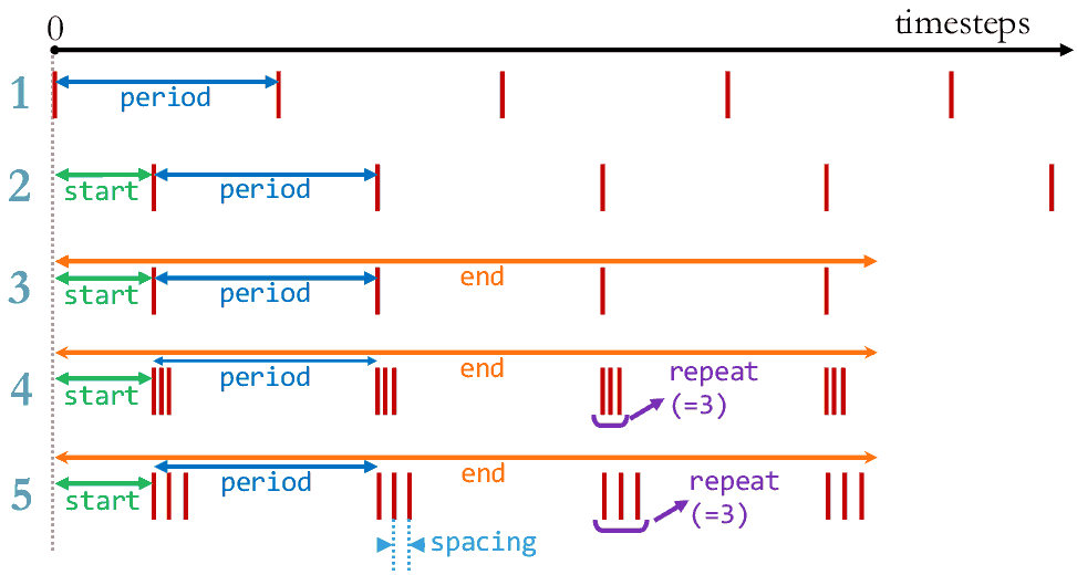
Tips
The syntax
every = periodis also accepted.Any value set to
0will be replaced by the default value.Special case:
every=0means no output.The numbers may be non-integers (apart from
repeat). The closest timesteps are chosen.
Profiles
Some of the quantities described in the previous sections can be profiles that depend on space and/or time. See the documentation on profiles for detailed instructions.
Checkpoints
The simulation state can be saved (dumped) at given times (checkpoints) in order to be later restarted at that point.
A few things are important to know when you need dumps and restarts.
Do not restart the simulation in the same directory as the previous one. Files will be overwritten, and errors may occur. Create a new directory for your restarted simulation.
Manage your disk space: each MPI process dumps one file, and the total can be significant.
The restarted runs must have the same namelist as the initial simulation, except the Checkpoints block, which can be modified.
Checkpoints(
    # restart_dir = "dump1",
    dump_step = 10000,
    dump_minutes = 240.,
    exit_after_dump = True,
    keep_n_dumps = 2,
)
Parameters to save the state of the current simulation
- dump_step
- Default:
0The number of timesteps between each dump. If
0, no dump is done.
- dump_minutes
- Default:
0.The number of minutes between each dump. If
0., no dump is done.May be used in combination with
dump_step.
- exit_after_dump
- Default:
TrueIf
True, the code stops after the first dump. IfFalse, the simulation continues.
- keep_n_dumps
- Default:
2This tells Smilei to keep, in the current run, only the last
ndumps. Older dumps will be overwritten.The default value,
2, saves one extra dump in case of a crash during the next dump.
- file_grouping
- Default:
0(no grouping)The maximum number of checkpoint files that can be stored in one directory. Subdirectories are created to accomodate for all files. This is useful on filesystem with a limited number of files per directory.
- dump_deflate
to do
Parameters to restart from a previous simulation
- restart_dir
- Default:
NoneThe directory of a previous run from which Smilei should restart. For the first run, do not specify this parameter.
This path must either absolute or be relative to the current directory.
Note
In many situations, the restarted runs will have the exact same namelist as the initial simulation, except this
restart_dirparameter, which points to the previous simulation folder. You can use the same namelist file, and simply add an extra argument when you launch the restart:
mpirun ... ./smilei mynamelist.py "Checkpoints.restart_dir='/path/to/previous/run'"
- restart_number
- Default:
NoneThe number of the dump (in the previous run) that should be used for the restart. For the first run, do not specify this parameter.
In a previous run, the simulation state may have been dumped several times. These dumps are numbered 0, 1, 2, etc. until the number
keep_n_dumps. In case multiple dumps are kept, the newest one will overwrite the oldest one. To restart the simulation from the most advanced point, specify the dump number corresponding to the newest that was created.
Variables defined by Smilei
Smilei passes the following variables to the python interpreter for use in the namelist. They should not be re-defined by the user!
- smilei_mpi_rank
The MPI rank of the current process.
- smilei_mpi_size
The total number of MPI processes.
- smilei_omp_threads
The number of OpenMP threads per MPI.
- smilei_total_cores
The total number of cores.
Note
These variables can be access during happi post-processing, e.g.
S.namelist.smilei_mpi_size.