Vectorization

For enhanced performances on most recent CPUs, Smilei exploits efficiently vectorization using refactored and optimized operators.

Vectorization optimizations are published in [Beck2019].

---

Notion of Single Instruction Multiple Data (SIMD) Vectorization

Single Instruction Multiple Data (SIMD) vectorization consists on performing on a contiguous set of data, usually called vector, the same operation(s) in a single instruction. On modern Computational Processing Units (CPU), vector registers have a length 512 kb that corresponds to 8 double precision floats (on Intel Skylake processors for instance and future ARM architecture). Each processing unit can perform a Fused Multiply Add instruction (FMA) that combines an addition and a multiplication. If-conditions can be handled using mask registers. Modern SIMD vectorization is described in Fig. 8.

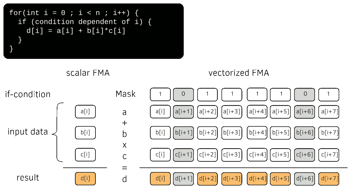
Fig. 8 Single Instruction Multiple Data (SIMD) vectorization

On SIMD CPUs, an application has to use SIMD vectorization to reach the maximum of the core computational peak performance. A scalar code without FMA uses less than 7% of the core computational power. This affirmation can nonetheless be mitigated on Intel Skylake processors that adapt their frequency on the used vectorization instruction set.

---

SIMD vectorization of the particle operators

Optimization efforts have been recently done to vectorize efficiently the particle operators of Smilei.

A new sorting method has been first implemented in order to then make the particle operator vectorization easier. This method, referred to as cycle sort, minimizes the number of data movements by performing successive permutation.

The most expensive operators and most difficult to vectorize are the current projection (deposition) and the field interpolation (gathering) steps where there is an interpolation between the grids and the macro-particles. These two steps have been vectorized taking advantage of the cycle sort.

---

Vectorization Performance

Vectorization is not always the most efficient choice. It depends on the number of macro-particles per cell. To demonstrate this, we have evaluated in [Beck2019] the performance with a series of tests on different architectures: Intel Cascade Lake, Intel Skylake, Intel Knights Landing, Intel Haswell, Intel Broadwell. The Cascade Lake processor is not in the original study and has been added after. We have used the 3D homogeneous Maxwellian benchmark available here. The number of macro-particles per cell is varied from 1 to 512. This study has been focused on the particle operators (interpolator, pusher, projector, sorting) and discards the computational costs of the Maxwell solver and of the communications between processes. Each run has been performed on a single node with both the scalar and the vectorized operators.. Since the number of cores varies from an architecture to another, the runs were conducted so that the load per core (i.e. OpenMP thread) is constant. The number of patches per core also remains the same for all cores throughout the whole simulation since the imbalance in this configuration is never high enough to trigger patch exchanges. The patch size is kept constant at 8 × 8 × 8 cells. The total number of patches for each architecture is determined so that each core has 8 patches to handle. The numerical parameters are given in Table 1.

Table 1 Numerical parameters for vectorization

Cluster	Architecture	Number of patches	Configuration
Jean Zay, IDRIS, France	2 x Cascade Lake (Intel® Xeon® Gold 6248, 20 cores)	5 x 8 x 8	Intel 19, IntelMPI 19
Irene Joliot-Curie, TGCC, France	2 x skylake (Intel® Skylake 8168, 24 cores)	6 x 8 x 8	Intel 18, IntelMPI 18
Frioul, Cines, France	2 x Knights Landing (Intel® Xeon® Phi 7250, 68 cores)	8 x 8 x 8	Intel 18, IntelMPI 18
Tornado, LPP, France	2 x Broadwell (Intel® Xeon® E5-2697 v4, 16 cores)	4 x 8 x 8	Intel 17, openMPI 1.6.5
Jureca, Juelich, Germany	2 x Haswell (Intel® Xeon® E5-2680 v3, 12 cores)	3 x 8 x 8	Intel 18, IntelMPI 18

The results of the simulation tests (shape factor of order 2) for both scalar and vectorized versions are shown in Fig. 9. Contrary to the scalar mode, the vectorized operators efficiency depends strongly on the number of particles per cell. It shows improved efficiency, compared to the scalar mode, above a certain number of particles per cell denoted inversion point.

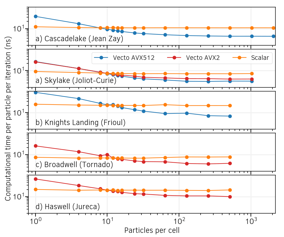
Fig. 9 Particle computational cost as a function of the number of particles per cell. Vectorized operators are compared to their scalar versions on various cluster architectures. Note that the Skylake compilations accepts both AVX512 and AVX2 instruction sets.

The lower performances of the vectorized operators at low particles per cell can be easily understood:

1. The complexity of vectorized algorithms is higher than their scalar counter-parts.

2. New schemes with additional loops and local buffers induced an overhead that is onmy compensated when the number of particles is large enough.

3. SIMD instructions are not efficient if not fulfilled

4. SIMD instructions operate at a lower clock frequency than scalar ones on recent architectures

The location of the inversion point of the speed-ups brought by vectorization depends on the architecture. The performance results are summarized in Table 2.

Table 2 Vectorization performance

Architecture (Cluster)	Inversion point (particles per cell)	Vectorization speed-up
Cascade lake (Jean Zay)	8 particles per cell	x2
Skylake (Irene Joliot-Curie)	10 particles per cell (most advanced instruction set)	x2.1
KNL (Frioul)	12 particles per cell	x2.8
Broadwell (LLR)	10 particles per cell	x1.9
Haswell (Jureca)	10 particles per cell	x1.9

Vectorization efficiency increases with the number of particles per cell above the inversion point. It tends to stabilize far from the inversion point above 256 particles per cell.

---

Adaptive vectorization

Adaptive vectorization consists on switching localy between scalar and vectorized operators during the simulation, choosing the most efficient one in the region of interest. The concept has been successfully implemented at the lower granularity of the code. Every given number of time steps, for each patch, and for each species, the most efficient set of operator is determined from the number of particles per cell. The concept is schematically described in Fig. 10.

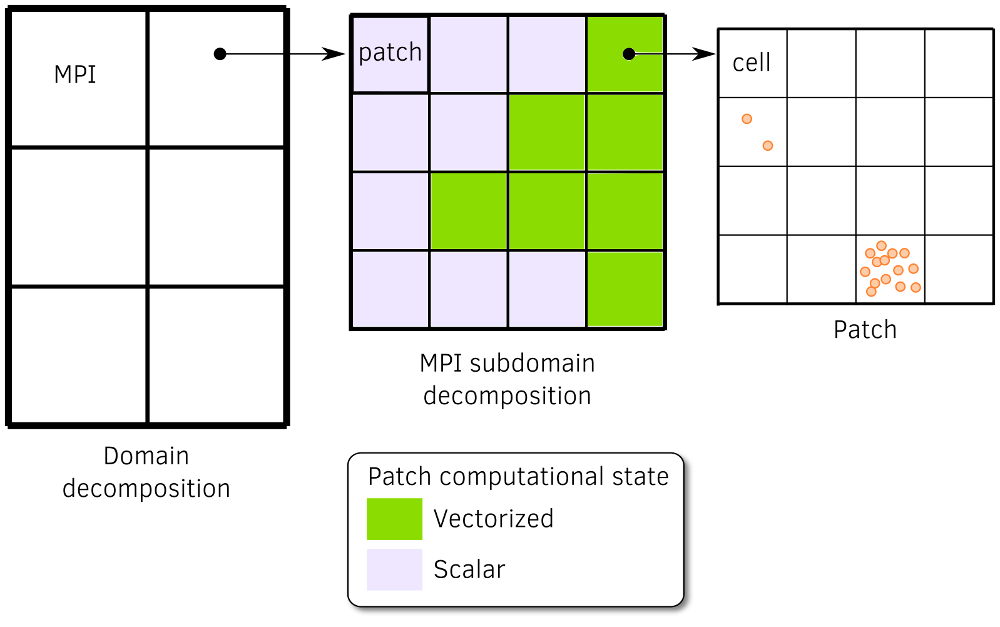
Fig. 10 Description of the adaptive vectorization withn the multi-stage domain decomposition. Patches with many macro-particles per cell are faster in with vectorized operators whereas with few macro-particles per cell, scalar operators are more efficient.

An advanced empirical criterion has been developed. It is computed from the parametric studies presented in Fig. 9 summarizes their results and indicates, for a given species in a given patch, the approximate time to compute the particle operators using both the scalar and the vectorized operator. The computation times have been normalized to that of the scalar operator for a single particle. The comparision of all normalized curves is presented in Fig. 11.

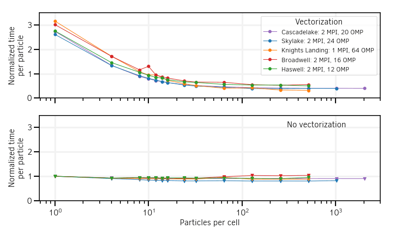
Fig. 11 Normalized time per particle spent for all particle operators in the scalar and vectorized modes with various architectures, and 2nd-order interpolation shape functions.

The outcomes from different architectures appear sufficiently similar to consider an average between their results. A linear regression of the average between all is applied on the scalar results to have a fit function to implement in the code. It writes:

(6)\[S(N) = -1.11 \times 10^{-2} \log{\left( N \right)} + 9.56 \times 10^{-1}\]

S is the computation time per particle normalized to that with 1 PPC, and N is the number of PPC. For the average between vectorized results, a fourth-order polynomial regression writes:

(7)\[\begin{split}V(N) = 1.76 \times 10^{ -3 } \log{ \left( N \right)}^4 \\ \nonumber + 8.41 \times 10^{ -2 } \log{ \left( N \right)}^3 \\ \nonumber + 1.45 \times 10^{ -2 } \log{ \left( N \right)}^2 \\ \nonumber -1.19 \log{ \left( N \right) } \\ \nonumber + 2.86\end{split}\]

The polynomial regressions are shown in Fig. 12.

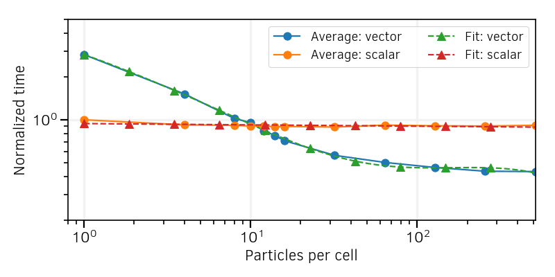
Fig. 12 Averages of the curves of Fig. 11 , and polynomial regressions.

These functions are implemented in the code to determine approximately the normalized single-particle cost. Assuming every particle takes the same amount of time, the total time to advance a species in a given patch can then be simply evaluated with a sum on all cells within the patch as:

(8)\[T_{\rm s,v} = \sum_{c \ \in\ patch\ cells} N(c) \times F\!\left(N(c)\right)\]

where F is either S or V. Comparing \(T_s\) and \(T_v\) determines which of the scalar or vectorized operators should be locally selected. This operation is repeated every given number of time steps to adapt to the evolving plasma distribution. Note that similar approximations may be computed for specific processors instead of using a general rule. In Smilei, other typical processors have been included, requiring an additional compilation flag automatically included in the machine files for make.

The process of computing the faster mode and changing operators accordingly is called reconfiguration

Large-scale simulations

Adaptive vectorization has been validated on large-scale simulations with different benchmarks. The following video enables to visualize on different scenarii the behavior of the adaptive vectorization.

Mildly-relativistic collisionless shock

One of the case was the simulation of Mildly-relativistic collisionless shock. The effect of the adaptive vectorization mode is illustrated by Fig. 13. The electron density is shown in the volume rendering of the top. The volume rendering at the bottom shows and patch computational state for the electron species.

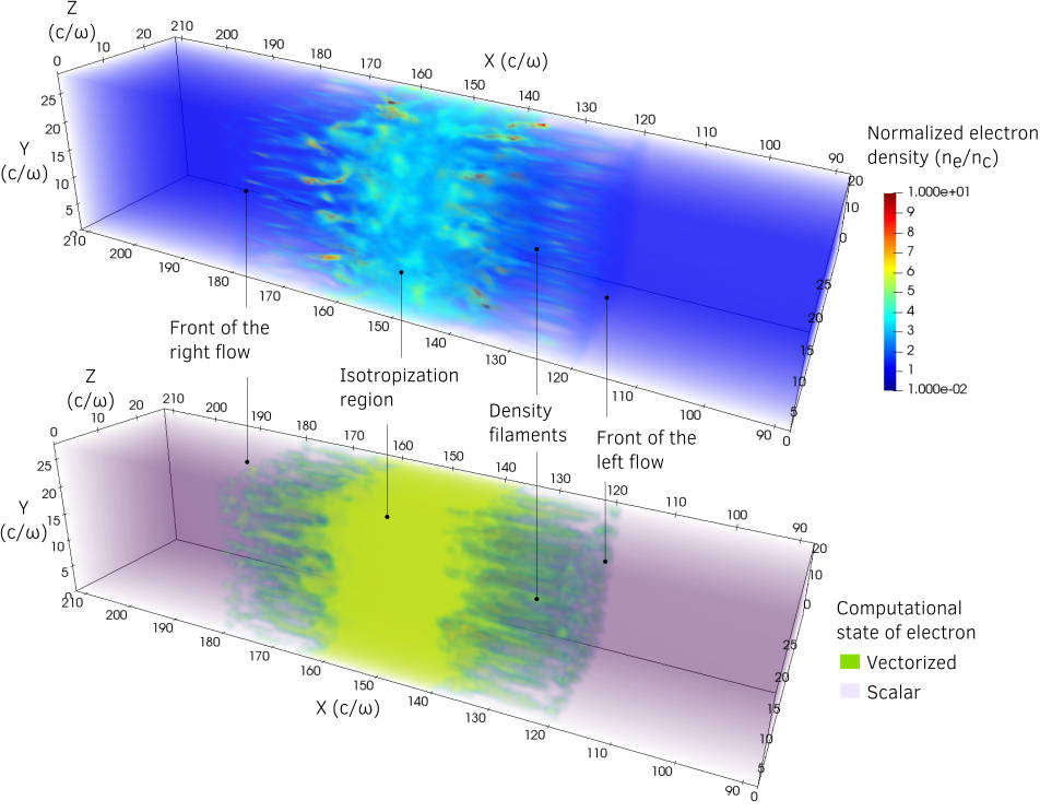
Fig. 13 Mildly-relativistic collisionless shock: On the top, volume rendering of the normalized electron density \(n_e /n_c\) (\(n_c\) the critical density) at time \(t = 34 \omega^{-1}\) (\(\omega\) the laser frequency) after the beginning of the collision. On the bottom, patches in vectorized mode for the electron species at the same time. An animated version of these can be viewed by clicking on this image.

Thanks to the adaptive vectorization, high-density regions that contains many macro-particles per cell corresponds to the patches in vectorized mode. Incoming plasma flows, with 8 particles per cell in average, are in scalar mode. The following video shows how the patches are dynamically switched in vectorized or scalar mode.

For this specific benchmark, the speed-up obtained with vectorization is of x2. Adaptive vectorization brinds a small additional speed-up in some cases.