Laser envelope model¶

In many physical situations, the spatial and temporal scales of interest (e.g. the plasma wavelength \(\lambda_p\)) are much larger than the scales related to the laser central wavelength \(\lambda_0\). In these cases, if the laser pulse is much longer than \(\lambda_0\), the computation time can be substantially reduced: one only needs to sample the laser envelope instead of \(\lambda_0\), as depicted in the following figure.

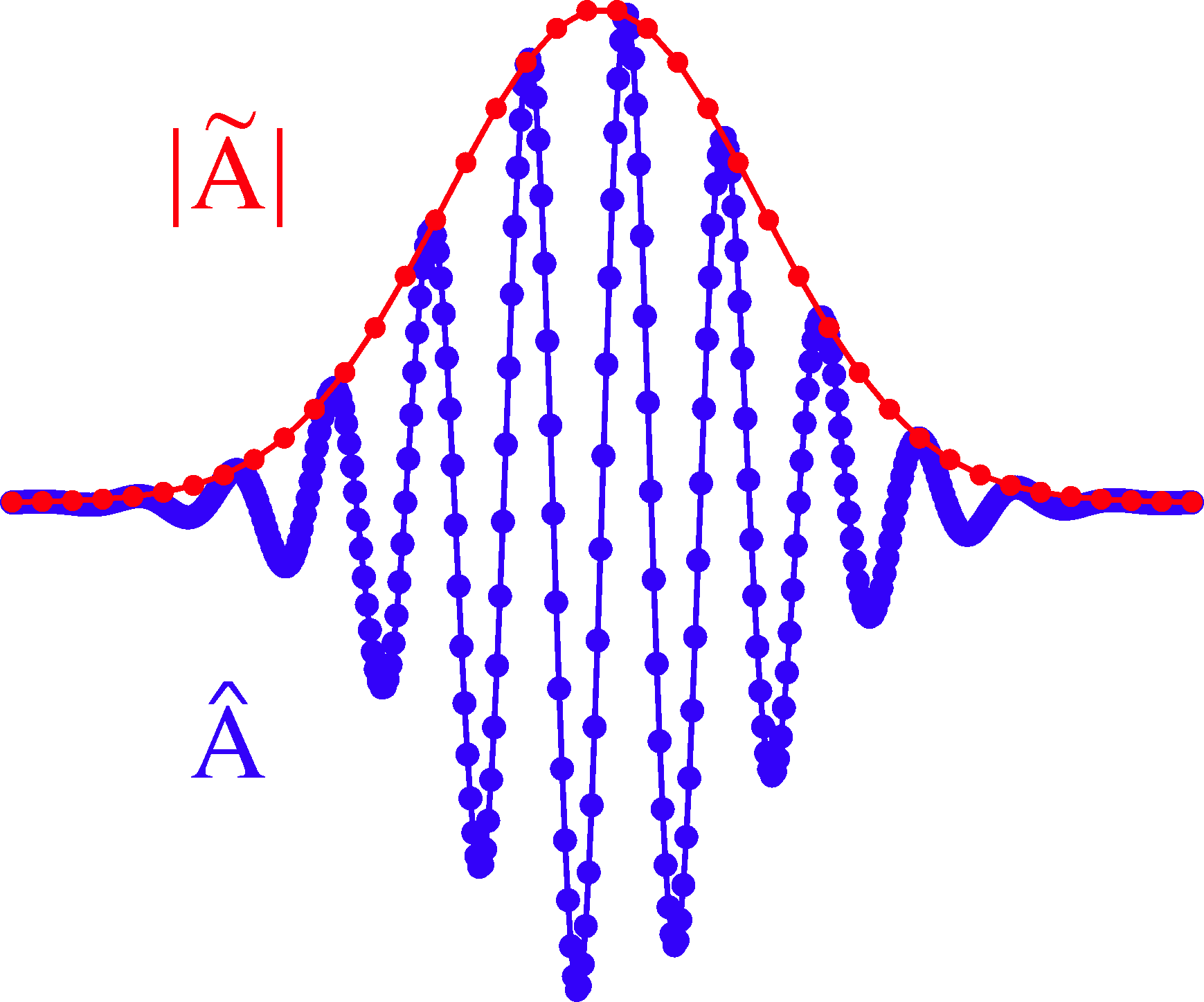
../_images/Envelope_Figure.png — Fig. 45 Blue: laser vector potential component \(\hat{A}\) along the transverse direction. Red: the module of its complex envelope \(|\tilde{A}|\). Both the lines display a suitable number of points for a proper sampling. In this case, the envelope is sampled by a number of points smaller by a factor ten.¶

The description of the physical system in terms of the complex envelope of the laser vector potential, neglecting its fast oscillations, is the essence of the envelope approximation. However, a main limit of this technique is the impossibility to model phenomena at the scale of \(\lambda_0\).

In the following, the equations of the envelope model are presented, following mainly [Cowan2011], [Terzani], [MassimoPPCF2019] . Their numerical solution is briefly described as well.

The envelope approximation¶

The use of envelope models to describe a laser pulse is well known in PIC codes [Mora1997], [Quesnel1998], [Gordon2000], [Huang2006], [Cowan2011], [Benedetti2012]. The basic blocks of a PIC code using an envelope description for the laser are an envelope equation, to describe the evolution of the laser, and equations of motion for the macro-particles, to take into account their interactions with the laser. The effect of the plasma on laser propagation is taken into account in the envelope equation through the plasma susceptibility, as described in the following section. The various PIC codes using an envelope model for the laser solve different versions of the envelope equation, depending mostly on which terms are retained and which ones are neglected, or the set of coordinates used to derive the envelope equation. Also the numerical schemes used to solve the envelope equation and the equations of motion of the macro-particles vary accordingly. In Smilei, the version of the envelope model written in laboratory frame coordinates, first demonstrated in the PIC code ALaDyn [Benedetti2008], [Terzani] is implemented, including the same numerical scheme to solve the lab frame coordinates envelope equation.

The basic assumption of the model is the description of the laser pulse vector potential in the transverse direction \(\mathbf{\hat{A}}(\mathbf{x},t)\) as a slowly varying envelope \(\mathbf{\tilde{A}}(\mathbf{x},t)\) modulated by fast oscillations at wavelength \(\lambda_0\), moving at the speed of light \(c\):

(48)¶\[\mathbf{\hat{A}}(\mathbf{x},t)=\textrm{Re}\left[\mathbf{\tilde{A}}(\mathbf{x},t)e^{ik_0(x-ct)}\right],\]

where \(k_0=2\pi/\lambda_0\). In the language of signal processing, \(\mathbf{\tilde{A}}\) is the complex envelope of \(\mathbf{\hat{A}}\). In other words, the spectral content of \(\mathbf{\tilde{A}}\) is given by the positive frequency components of \(\mathbf{\hat{A}}\) around \(k_0\), but centered around the origin of the frequency \(k\) axis. As the laser is the source term of the phenomena of interest, in general any vector \(\mathbf{A}\) will be therefore given by the summation of a slowly varying part \(\mathbf{\bar{A}}\) and a fast oscillating part \(\mathbf{\hat{A}}\) with the same form of Eq. (48):

\[\mathbf{A}=\mathbf{\bar{A}} + \mathbf{\hat{A}}.\]

In the envelope model context, “slowly varying” means that the spatial and temporal variations of \(\mathbf{\bar{A}}\) and \(\mathbf{\tilde{A}}\) are small enough to be treated perturbatively with respect to the ratio \(\epsilon=\lambda_0/\lambda_p\), as described in detail in [Mora1997], [Quesnel1998], [Cowan2011]. The laser envelope transverse size \(R\) and longitudinal size \(L\) are thus assumed to scale as \(R \approx L \approx \lambda_0 / \epsilon\) [Mora1997], [Quesnel1998]. As described thoroughly in the same references, the coupling between the laser envelope and the plasma macro-particles can be modeled through the addiction of a ponderomotive force term in the macro-particles equations of motion. This term, not representing a real force, is a term rising from an averaging process in the perturbative treatment of the macro-particles motion over the laser optical cycles.

Modeling the laser through a complex envelope and its coupling with the plasma through the ponderomotive force will yield physically meaningful results only if the variation scales in space and time are greater than \(\lambda_0\), \(1/\omega_0\). Examples violating these hypotheses include, but are not limited to, tightly focused lasers, few optical cycles lasers, sharp gradients in the plasma density.

The envelope equation¶

The evolution of the laser pulse is described by d’Alembert’s equation, which in normalized units reads:

(49)¶\[\nabla^2 \mathbf{\hat{A}}-\partial^2_t\mathbf{\hat{A}}=-\mathbf{\hat{J}},\]

where \(\mathbf{\hat{J}}\) is the fast oscillating part of the current density in the laser polarization direction. Through the assumption given by Eq. (48), Eq. (49) can be reduced to an envelope equation:

(50)¶\[\nabla^2 \mathbf{\tilde{A}}+2i\left(\partial_x \mathbf{\tilde{A}} + \partial_t \mathbf{\tilde{A}}\right)-\partial^2_t\mathbf{\tilde{A}}=\chi \mathbf{\tilde{A}},\]

which describes the evolution of the laser pulse only in terms of the laser envelope \(\mathbf{\tilde{A}}\). The function \(\chi\) represents the plasma susceptibility, which is computed similarly to the charge density (see PIC algorithms) as

(51)¶\[\chi(\mathbf{x}) = \sum_s\,\frac{q^2_s}{m_s}\,\sum_p\,\frac{w_p}{\bar{\gamma}_p}\,S\big(\mathbf{x}-\mathbf{\bar{x}}_p\big)\,\]

where \(\bar{\gamma}_p\) is the averaged Lorentz factor of the macro-particle \(p\). This averaged quantity is computed from the averaged macro-particle momentum \(\mathbf{\bar{u}}_p=\mathbf{\bar{p}}_p/m_s\) and the envelope \(\mathbf{\tilde{A}}\):

(52)¶\[\bar{\gamma}_p = \sqrt{1+\mathbf{\bar{u}}^2_p+\frac{|\mathbf{\tilde{A}}(\mathbf{\bar{x}}_p)|^2}{2}}.\]

The term at the right hand side of Eq. (48), where the plasma susceptibility \(\chi\) appears, allows to describe phenomena where the plasma alters the propagation of the laser pulse, as relativistic self-focusing.

Note that if in Eq. (48) the temporal variation of the envelope \(\mathbf{\tilde{A}}\) is neglected, and \(\partial^2_x \mathbf{\tilde{A}} \ll 2i\partial_x \mathbf{\tilde{A}}\) is assumed, the well-known paraxial wave equation is retrieved in vacuum (\(\chi=0\)):

(53)¶\[\nabla_{\perp}^2 \mathbf{\tilde{A}}+2i\partial_x \mathbf{\tilde{A}}=0.\]

In Smilei, no assumptions on the derivatives are made and the scalar versions of Eq. (50) is solved (see next sections).

The ponderomotive equations of motion¶

The process of averaging over the time scale of a laser oscillation period yields a simple result for the macro-particles equations of motion. The averaged position \(\mathbf{\bar{x}}_p\) and momentum \(\mathbf{\bar{u}}_p\) of the macro-particle \(p\) are related to the averaged electromagnetic fields \(\mathbf{\bar{E}}_p=\mathbf{\bar{E}}(\mathbf{\bar{x}}_p)\), \(\mathbf{\bar{B}}_p=\mathbf{\bar{B}}(\mathbf{\bar{x}}_p)\) through the usual equations of motion, with the addition of a ponderomotive force term which models the interaction with the laser:

(54)¶\[\begin{split}\begin{eqnarray} \frac{d\mathbf{\bar{x}}_p}{dt} &=& \frac{\mathbf{\bar{u}_p}}{\bar{\gamma}_p}, \,\\ \frac{d\mathbf{\bar{u}}_p}{dt} &=& r_s \, \left( \mathbf{\bar{E}}_p + \frac{\mathbf{\bar{u}}_p}{\bar{\gamma}_p} \times \mathbf{\bar{B}}_p \right)-r^2_s\thinspace\frac{1}{4\bar{\gamma}_p}\nabla\left(|\mathbf{\tilde{A}}_p|^2\right), \end{eqnarray}\end{split}\]

where \(r_s = q_s/m_s\) is the charge-over-mass ratio (for species \(s\)). The presence of the ponderomotive force \(\mathbf{F}_{pond}=-r^2_s\thinspace\frac{1}{4\bar{\gamma}_p}\nabla\left(|\mathbf{\tilde{A}}|^2\right)\) and of the ponderomotive potential \(\Phi_{pond}=\frac{|\mathbf{\tilde{A}}|^2}{2}\) in the envelope and particle equations is the reason why the envelope model is also called ponderomotive guiding center model [Gordon2000].

The averaged electromagnetic fields¶

In the envelope model, Maxwell’s equations remain unaltered, except for the fact that they describe the evolution of the averaged electromagnetic fields \(\mathbf{\bar{E}}(\mathbf{x},t)\), \(\mathbf{\bar{B}}(\mathbf{x},t)\) in terms of the averaged charge density \(\bar{\rho}(\mathbf{x},t)\) and averaged current density \(\mathbf{\bar{J}}(\mathbf{x},t)\):

(55)¶\[\begin{split}\begin{eqnarray} \nabla \cdot \mathbf{\bar{B}} &=& 0 \,,\\ \nabla \cdot \mathbf{\bar{E}} &=& \bar{\rho} \,,\\ \nabla \times \mathbf{\bar{B}} &=& \mathbf{\bar{J}} + \partial_t \mathbf{\bar{E}} \,,\\ \nabla \times \mathbf{\bar{E}} &=& -\partial_t \mathbf{\bar{B}} \,. \end{eqnarray}\end{split}\]

Note that the averaged electromagnetic fields do not include the laser fields. Thus, also in the diagnostics of Smilei, the fields will include only the averaged fields.

The ponderomotive PIC loop¶

Since Maxwell’s equations (55) remain unaltered, their solution can employ the same techniques used in a standard PIC code. The main difficulty in the solution of the other equations, namely the envelope equation Eq. (50) and the macroparticles equations of motion Eqs. (54), is that the source terms contain the unknown terms. For example, in the envelope equations, the source term involves the unknown envelope itself and the susceptibility, which depends on the envelope. Also, the equations of motion contain the term \(\bar{\gamma}\), which depends on the envelope. The PIC loop described in PIC algorithms is thus modified to self-consistently solve the envelope model equations. At each timestep, the code performs the following operations

interpolating the electromagnetic fields and the ponderomotive potential at the macro-particle positions,
projecting the new plasma susceptibility on the grid,
computing the new macro-particle velocities,
computing the new envelope values on the grid,
computing the new macro-particle positions,
projecting the new charge and current densities on the grid,
computing the new electromagnetic fields on the grid.

Note that the momentum advance and position advance are separated by the envelope equation solution in this modified PIC loop. In this section, we describe these steps which advance the time from time-step \((n)\) to time-step \((n+1)\).

Field interpolation¶

The electromagnetic fields and ponderomotive potential interpolation at the macro-particle position at time-step \((n)\) follow the same technique described in PIC algorithms:

\[\begin{split}\begin{eqnarray} \mathbf{\bar{E}}_p^{(n)} = V_c^{-1} \int d\mathbf{x}\, S\left(\mathbf{x}-\mathbf{\bar{x}}_p^{(n)}\right) \mathbf{\bar{E}}^{(n)}(\mathbf{x})\,,\\ \mathbf{\bar{B}}_p^{(n)} = V_c^{-1} \int d\mathbf{x}\, S\left(\mathbf{x}-\mathbf{\bar{x}}_p^{(n)}\right) \mathbf{\bar{B}}^{(n)}(\mathbf{x})\,,\\ \mathbf{\Phi}_p^{(n)} = V_c^{-1} \int d\mathbf{x}\, S\left(\mathbf{x}-\mathbf{\bar{x}}_p^{(n)}\right) \mathbf{\Phi}^{(n)}(\mathbf{x})\,, \end{eqnarray}\end{split}\]

where we have used the time-centered magnetic fields \(\mathbf{\bar{B}}^{(n)}=\tfrac{1}{2}[\mathbf{\bar{B}}^{(n+1/2) } + \mathbf{\bar{B}}^{(n-1/2)}]\), and \(V_c\) denotes the volume of a cell.

Susceptibility deposition¶

The macro-particle averaged positions \(\mathbf{\bar{x}}_p^{(n)}\) and averaged momenta \(\mathbf{\bar{p}}_p^{(n)}\) and the ponderomotive potential \(\mathbf{\Phi}_p^{(n)}\) are used to compute the ponderomotive Lorentz factor \(\bar{\gamma}_p\) (52) and deposit the susceptibility on the grid through Eq. (51).

Ponderomotive momentum push¶

The momentum push is performed through a modified version of the well-known Boris Pusher, derived and proposed in [Terzani]. The plasma electric, magnetic and ponderomotive potential fields at the macro-particle position \(\mathbf{\bar{E}}_p^{(n)}\), \(\mathbf{\bar{B}}_p^{(n)}\), \(\mathbf{\Phi}_p^{(n)}\) are used to advance the momentum \(\mathbf{\bar{p}}_p^{(n-1/2)}\) from time-step \(n−1/2\) to time-step \(n + 1/2\), solving the momentum equation in Eqs. (54)

Envelope equation solution¶

Now that the averaged susceptibility is known at time-step \(n\), the envelope can be advanced solving the envelope equation (50). In the two solver schemes available in the code (see below), the envelope \(\mathbf{\tilde{A}}\) at time-step \(n+1\) is computed from its value at timesteps \(n\), \(n-1\) and the suceptibility \(\chi\) at time-step \(n\). The value of the envelope at timestep \(n\) is conserved for the next iteration of the time loop. A main advantage of these explicit numerical schemes is their straightforward parallelization in 3D, due to the locality of the operations involved.

Ponderomotive position push¶

The updated ponderomotive potential is interpolated at macro-particle positions to obtain \(\mathbf{\Phi}_p^{(n+1)}\). Afterwards, the temporal interpolation \(\mathbf{\Phi}_p^{(n+1/2)}=\left(\mathbf{\Phi}_p^{(n)}+\mathbf{\Phi}_p^{(n+1)}\right)/2\) is performed. The updated ponderomotive Lorentz factor \(\bar{\gamma}_p^{(n+1/2)}\) can be computed and the averaged position of each macro-particle can be advanced solving the last of Eqs. (54):

\[\mathbf{\bar{x}}_p^{n+1}=\mathbf{\bar{x}}_p^{n} + \Delta t \, \frac{\mathbf{\bar{p}}_p^{n+\tfrac{1}{2}}}{m_s\bar{\gamma}_p^{(n+1/2)}},\]

Current deposition¶

The averaged charge deposition (i.e. charge and current density projection onto the grid) is then performed exactly as in the standard PIC loop for the non averaged quantities (see PIC algorithms), using the charge-conserving algorithm proposed by Esirkepov.

Maxwell solvers¶

Now that the averaged currents are known at time-step \(n+\tfrac{1}{2}\), the averaged electromagnetic fields can be advanced solving Maxwell’s equations (55). Their solution is identical to the one described in PIC algorithms for the corresponding non-averaged quantities.

Laser polarization in the envelope model¶

In Smilei, the envelope model is implemented to take into account either linear or circular polarization (ellipticity = 0 and ellipticity = 1 in the input namelist respectively). The default polarization is linear along the y direction. The envelope of a laser pulse propagating in the positive x direction can be written as

\[\mathbf{\tilde{A}} (\mathbf{x},t)= \tilde{A}(\mathbf{x},t) \left[ \eta\thinspace\hat{y} + i(1-\eta^2)^{1/2}\hat{z} \right] ,\]

where \(\eta=1\) or \(\eta=0\) for linear polarization along y or z, and \(\eta\pm1/\sqrt{2}\) for circular polarization. Although Eq. (50) is a vector equation nonlinear, these two polarizations allow to solve only one scalar equation at each timestep, because once the susceptibility at a given timestep is known, the envelope equation can be considered linear. Thus, after calculating the susceptibility we can solve the equation:

(56)¶\[\nabla^2 \tilde{A}+2i\left(\partial_x \tilde{A} + \partial_t \tilde{A}\right)-\partial^2_t\tilde{A}=\chi \tilde{A},\]

where \(\tilde{A}\) is the nonzero component of \(\mathbf{\tilde{A}}\) for linear polarization and \(\tilde{A}/\sqrt{2}\) for circular polarization. This approach gives accurate results only if the ponderomotive potential \(\Phi_{pond}=\frac{|\mathbf{\tilde{A}}|^2}{2}\) is computed accordingly to the vector definition of \(\mathbf{\tilde{A}}\). This means that \(\Phi_{pond}=\frac{|\tilde{A}|^2}{2}\) for both linear and circular polarization. Besides, with this approach the absolute value of \(\tilde{A}\) and the derived electric field \(\tilde{E}\) (see next section) are directly comparable with standard laser simulations with the same polarization and \(a_0\).

Computing the laser electric field from the laser envelope¶

It is always useful (and recommendable) to compare the results of an envelope simulation and of a standard laser simulation, to check if the envelope approximation is suitable for the physical case that is simulated. For this purpose, the plasma electromagnetic fields and the charge densities are easily comparable. However, in an envelope simulation all the plasma dynamics is written as function of the envelope of the transverse component of the vector potential \(\tilde{A}\), as explained in the previous sections, and not as function of the laser electric field.

Furthermore, in case of envelope simulations with ionization, the ionization rate formula is computed using the electric field (longitudinal and transverse components) of the laser.

For these two reasons (diagnostic and ionization), in an envelope simulation two additional fields are computed, \(\tilde{E}\) and \(\tilde{E_x}\), which represent respectively the envelope of the transverse component and of the longitudinal component of the laser electric field.

From Eq. (48), the laser transverse electric field’s complex envelope \(\tilde{E}\) can be derived. In the context of the perturbative treatment, the laser scalar potential can be neglected [Cowan2011], yielding:

\[\hat{E} = -\partial_t \hat{A} = -\partial_t \Big\{\textrm{Re}\left[\tilde{A}(\mathbf{x},t)e^{ik_0(x-ct)}\right]\Big\} = \textrm{Re}\left[-\left(\partial_t-ik_0c\right)\tilde{A}(\mathbf{x},t)e^{ik_0(x-ct)}\right],\]

which can be expressed, following the definition in Eq. (48), also as

\[\hat{E} = \textrm{Re}\left[\tilde{E}(\mathbf{x},t)e^{ik_0(x-ct)}\right].\]

The laser transverse electric field’s complex envelope \(\tilde{E}\) can thus be defined:

\[\tilde{E} = -\left(\partial_t-ik_0c\right)\tilde{A}(\mathbf{x},t).\]

In the same theoretical framework, it can be shown that the laser longitudinal electric field’s envelope can be computed through a partial derivative along the direction perpendicular to the laser propagation direction:

\[\tilde{E_x} = -\partial_{\perp}\tilde{A}(\mathbf{x},t).\]

In the diagnostics, the absolute value of the fields \(\tilde{E}\), \(\tilde{E_x}\) are available, under the names Env_E_abs and Env_Ex_abs.

The numerical solution of the envelope equation¶

To solve Eq. (56), two explicit numerical schemes are implemented in the code, first implemented in the PIC code ALaDyn [Benedetti2008] and described in [Terzani].

In the first scheme, denoted as "explicit" in the input namelist, the well known central finite differences are used to discretize the envelope equation. In 1D for example, the spatial and time derivatives of the envelope \(\tilde{A}\) at time-step \(n\) and spatial index \(i\) are thus approximated by:

\[\begin{split}D_x\tilde{A}\bigg\rvert^{n}_{i}&=&\frac{\tilde{A}^n_{i+1}-\tilde{A}^n_{i-1}}{2\Delta x},\\ D_t\tilde{A}\bigg\rvert^{n}_{i}&=&\frac{\tilde{A}^{n+1}_{i}-\tilde{A}^{n-1}_{i}}{2\Delta t},\\ D_{xx}\tilde{A}\bigg\rvert^{n}_{i}&=&\frac{\tilde{A}^n_{i+1}-2\tilde{A}^n_{i}+\tilde{A}^n_{i-1}}{\Delta x^2},\\ D_{tt}\tilde{A}\bigg\rvert^{n}_{i}&=&\frac{\tilde{A}^{n+1}_{i}-2\tilde{A}^n_{i}+\tilde{A}^{n-1}_{i}}{\Delta t^2},\end{split}\]

where \(\Delta x, \Delta t\) are the cell size in the x direction and the integration time-step respectively.

In the second scheme, denoted as "explicit_reduced_dispersion" in the input namelist, the finite difference approximations for the derivatives along the propagation direction x are substituted by optimized finite differences that reduce the numerical dispersion in that direction (see [Terzani] for the derivation). Namely, defining \(\nu=\Delta t/\Delta x\), \(\delta=(1-\nu^2)/3\), these optimized derivatives can be written as:

\[\begin{split}D_{x,opt}\tilde{A}\bigg\rvert^{n}_{i}&=& (1+\delta)D_x\tilde{A}\bigg\rvert^{n}_{i}-\delta\left(\frac{\tilde{A}^n_{i+2}-\tilde{A}^n_{i-2}}{4\Delta x}\right),\\ D_{xx,opt}\tilde{A}\bigg\rvert^{n}_{i}&=& (1+\delta)D_{xx}\tilde{A}\bigg\rvert^{n}_{i}-\delta\left(\frac{\tilde{A}^n_{i+2}-2\tilde{A}^n_{i}+\tilde{A}^n_{i-2}}{4\Delta x^2}\right).\\\end{split}\]

In both schemes, after substituting the spatial and temporal derivative with the chosen finite differences forms, an explicit update of \(\tilde{A}^{n+1}_i\), function of \(\tilde{A}^{n}_i\), \(\tilde{A}^{n}_{i-1}\), \(\tilde{A}^{n}_{i+1}\), \(\tilde{A}^{n-1}_i\) and \(\chi^{n}_i\) can be easily found. In the reduced dispersion scheme, also the values \(\tilde{A}^{n}_{i-2}\), \(\tilde{A}^{n}_{i+2}\) are necessary for the update. The locality of the abovementioned finite difference stencils allows a parallelization with well known techniques and the extension to the other geometries is straightforward. The discretization of the transverse components of the Laplacian in Eq. (50) in Cartesian geometry uses the central finite differences defined above, applied to the y and z axes. In cylindrical geometry (see Azimuthal modes decomposition), the transverse part of the Laplacian is discretized as:

\[D^2_{\perp, cyl}\tilde{A}\rvert^{n}_{i,j} = \frac{\tilde{A}^n_{i,j+1}-2\tilde{A}^n_{i,j}+\tilde{A}^n_{i,j-1}}{\Delta r^2} + \frac{1}{r_j}\frac{\tilde{A}^n_{i,j+1}-\tilde{A}^n_{i,j-1}}{2\Delta r},\]

where \(j, r, \Delta r\) are the transverse index, the distance from the propagation axis and the radial cell size respectively.