Azimuthal modes decomposition

Smilei can run in cyclindrical geometry with a decomposition in azimuthal modes (AM), as described in this article. This requires a system with cylindrical symmetry or close to cylindrical symmetry (around the x axis in Smilei).

---

Mathematical definition

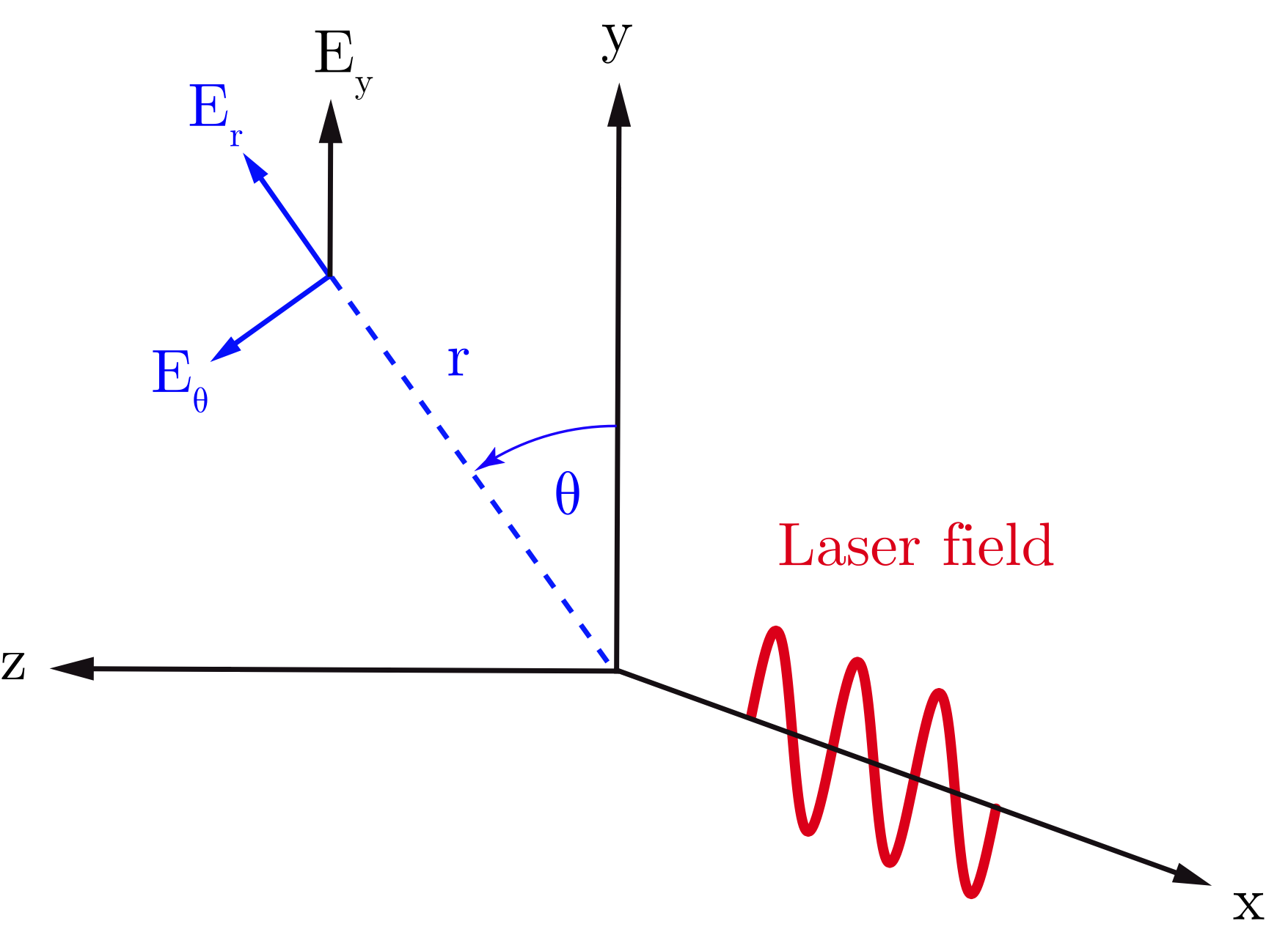
Fig. 41 Coordinates in azimuthal geometry.

Any scalar field \(F(x,r,\theta)\) can be decomposed into a basis of azimuthal modes, or harmonics, defined as \(\exp(-im\theta)\), where \(m\) is the number of the mode. Writing each Fourier coefficient as \(\tilde{F}^{m}\) leads to:

(41)\[F\left(x,r,\theta\right) = \textrm{Re}\left[ \sum_{m=0}^{+\infty}\tilde{F}^{m}\left(x,r\right)\exp{\left(-im\theta\right)} \right],\]

The mode \(m=0\) has cylindrical symmetry (no dependence on \(\theta\)). The following figure shows the real part of the first four azimuthal modes.

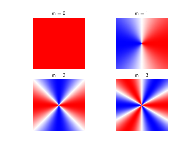
Fig. 42 Real part of the first four pure azimuthal modes \(exp(-im\theta)\) on the yz plane.

Eq. (41) can be expanded as:

(42)\[F\left(x,r,\theta\right) = \tilde{F}^{0}_{real} + \tilde{F}^{1}_{real}\cos(\theta) + \tilde{F}^{1}_{imag}\sin(\theta) + \tilde{F}^{2}_{real}\cos(2\theta) + \tilde{F}^{2}_{imag}\sin(2\theta) + ...\]

The complex coefficients \(\tilde{F}^{m}\) can be calculated from \(F\) according to:

\[\begin{split}\tilde{F}^{m} &=& \frac{1}{\pi}\int_0^{2\pi} F\left(x,r,\theta\right)\exp{\left(-im\theta\right)}d\theta & \quad\textrm{ for } m>0 \\ \tilde{F}^{0} &=& \frac{1}{2\pi}\int_0^{2\pi}F\left(x,r,\theta\right)d\theta. & \textrm{ for } m=0\end{split}\]

---

Decomposition of vector fields

Vector fields can also be decomposed in azimuthal modes through a decomposition of each of their components along the cylindrical coordinates \((\mathbf{e_x},\mathbf{e_r},\mathbf{e_\theta})\). For example, the transverse field \(\mathbf{E}_\perp\) of a laser pulse polarized in the \(y\) direction with cylindrically symmetric envelope can be written as

\[\begin{split}\mathbf{E}_\perp(x,r,\theta, t) &= E_y(x,r,\theta, t) \mathbf{e_y} \\ &= E_r (x,r,\theta, t) \mathbf{e_r} + E_{\theta}(x,r,\theta, t) \mathbf{e_{\theta}}\\ &= E_y(x,r,t) [\cos(\theta) \mathbf{e_r} - \sin(\theta) \mathbf{e_{\theta}}].\end{split}\]

Thus, comparing to Eq (42), we recognize a pure azimuthal mode of order \(m=1\) for both \(E_r\) and \(E_\theta\), with the Fourier coefficients:

\[ \begin{align}\begin{aligned}\begin{split}\tilde{E}^1_r (x,r,t) = E_y(x,r,t),\\\end{split}\\\tilde{E}^1_{\theta} (x,r,t) = -iE_y(x,r,t).\end{aligned}\end{align} \]

Similarly, an elliptically (or cylindrically) polarized laser is described by a pure mode \(m=1\), as it can be seen as the linear superposition of two linearly polarized lasers. A difference in phase or in the polarization direction simply corresponds to a multiplication of the Fourier coefficients by a complex exponential.

The AM decomposition is most suited for physical phenomena close to cylindrical symmetry as a low number of modes is sufficient. For example, in a basic Laser Wakefield Acceleration setup, a linearly-polarized laser pulse with cylindrically symmetric envelope may be described only by the mode \(m=1\). As the wakefield wave is mainly determined by the cylindrically symmetric ponderomotive force, it can be described by the mode \(m=0\). Thus, such a simulation only needs, in principle, two azimuthal modes.

---

Maxwell’s equations in cylindrical geometry

In an AM simulation, the \(\tilde{F}^{m}(x,r)\) are stored and computed for each scalar field and for each component of the vector fields. Each of them is a \((x,r)\) grid of complex values.

From the linearity of Maxwell’s Equations, and assuming that the densities and currents can also be decomposed in modes, we obtain the following evolution of the mode \(m\):

(43)\[\begin{split}\partial_t \tilde{B}^m_{x} &=-\frac{1}{r}\partial_r(r\tilde{E}^m_{\theta})-\frac{im}{r}\tilde{E}^m_r,\\ \partial_t \tilde{B}^m_r &= \frac{im}{r}\tilde{E}^m_x+\partial_x \tilde{E}^m_{\theta},\\ \partial_t \tilde{B}^m_{\theta} &=-\partial_x \tilde{E}^m_{r} + \partial_r \tilde{E}^m_{x},\\ \partial_t \tilde{E}^m_{x} &=\frac{1}{r}\partial_r(r\tilde{B}^m_{\theta})+\frac{im}{r}\tilde{B}^m_r-\tilde{J}^m_{x},\\ \partial_t \tilde{E}^m_r &= -\frac{im}{r}\tilde{B}^m_x-\partial_x \tilde{B}^m_{\theta}-\tilde{J}^m_{r},\\ \partial_t \tilde{E}^m_{\theta} &=\partial_x \tilde{B}^m_{r} - \partial_r \tilde{B}^m_{x}-\tilde{J}^m_{\theta}.\end{split}\]

Thus, even in presence of a plasma, at each timestep, these equations are solved independently. The coupling between the modes occurs when the total electromagnetic fields push the macro-particles, creating, in turn, the currents \(\tilde{J}^m\) of their current density.

---

Interaction with the macro-particles

The azimuthal decomposition concerns only the grid quantities (EM fields and current densities), which are thus defined on a 2D grid, but macro-particles evolve in a full three-dimensional space with cartesian coordinates.

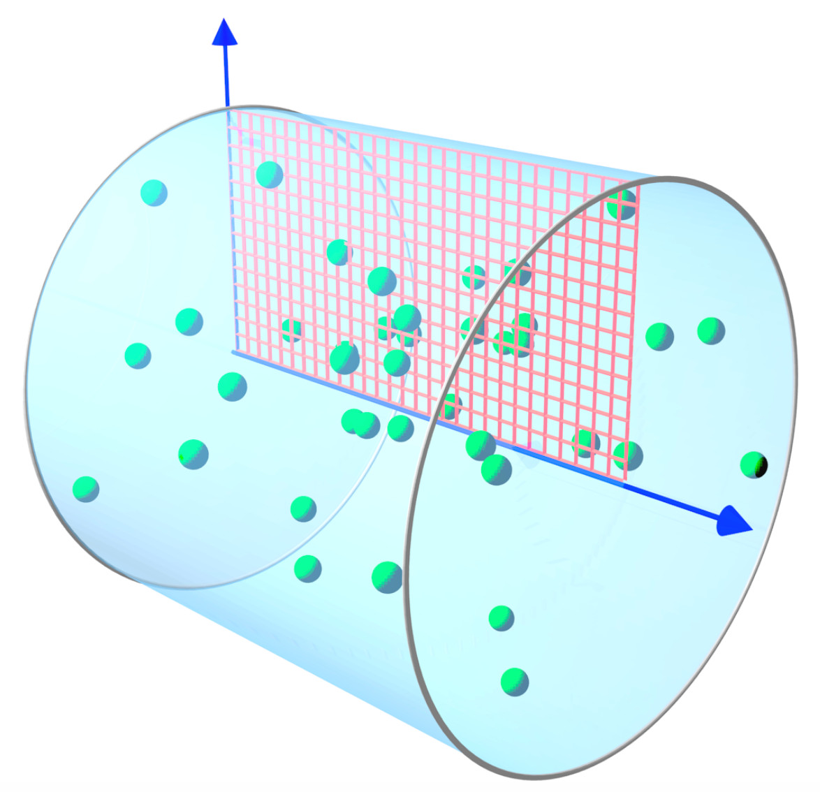
Fig. 43 Blue arrows: the x and r axes of the 2D grid (red) where the electromagnetic fields are defined. Macro-particle positions and momenta are defined in 3D.

During each iteration, the macro-particles are pushed in phase space using reconstructed 3D cartesian electromagnetic fields at their position \((x,r,\theta)\) (see Eq. (41)). Then, their contribution to the current densities \((J_x,J_r,J_{\theta})\) is computed to update the electromagnetic fields at the next iteration (see Eqs (43)).

---

Tips

Note that each mode \(\tilde{F}^{m}\) is a function of \(x\), the longitudinal coordinate and \(r\), the radial coordinate. Therefore, each of them is only two dimensional. Thus, the computational cost of AM simulations scales approximately as 2D simulations multiplied by the number of modes. However, a higher number of macro-particles might be necessary to obtain convergence of the results (always check the convergence of your results by increasing the number of macro-particles and modes). A rule of thumb is to use at least 4 times the number of modes as macro-particles along \(\theta\).

---

Conventions for the namelist

Several differences appear in the notations and definitions between the AM and 3D geometries:

• The origin of the coordinates is on the axis of the cylinder (see figure below).

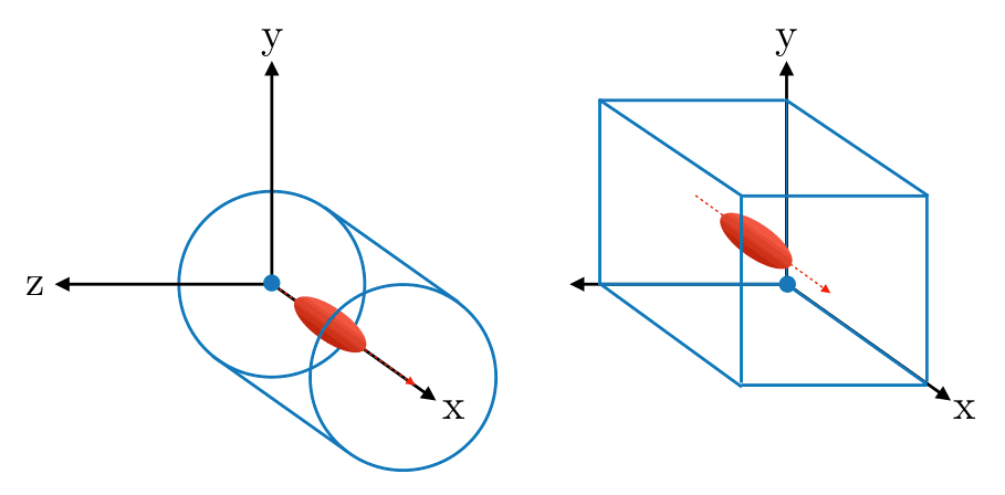
Fig. 44 Origin of coordinates in AM cylindrical and 3D cartesian.

• The AM radial grid size (grid_length[1]) represents the radius of the cylinder; not its diameter. Thus, it is half the size of the 3D transverse grid.

• Particles are defined 3D space, so their coordinates should be provided in terms of x, y, z if needed (e.g. a Species initialized with a numpy array). However, the density profiles of particles are assimilated to scalar fields defined on the \((x,r)\) grid.

• Field diagnostics really correspond to the complex fields of each mode on \((x,r)\) grids. However, Probes diagnostics are defined in 3D space just like the particles: all fields are interpolated at their 3D positions, and reconstructed by summing over the modes.

• ExternalFields are grid quantities in \((x,r)\) coordinates. One must be defined for each mode.

---

Classical and relativistic Poisson’s equation

Given the linearity of the relativistic Poisson’s equation described in Field initialization for relativistic species, it can be decomposed in azimuthal modes with the corresponding mode of the charge density \(-\tilde{\rho}^m\) as source term. For the mode m of the potential \(\Phi\), it writes:

(44)\[\left[ \frac{1}{\gamma^2_0}\partial^2_x\tilde{\Phi}^m +\frac{1}{r}\partial_r\left(r\partial_r\tilde{\Phi}^m\right) -\frac{m^2}{r^2}\tilde{\Phi}^m \right] = -\tilde{\rho}^m.\]

By solving each of these relativistic Poisson’s equations we initialize the azimuthal components of the electromagnetic fields:

\[\begin{split}\begin{eqnarray} \tilde{E}^m_x &=& -\frac{1}{\gamma_0^2}\partial_x \tilde{\Phi}^m,\\ \tilde{E}^m_r &=& -\partial_r \tilde{\Phi}^m, \\ \tilde{E}^m_{\theta} &=& \frac{im}{r} \tilde{\Phi}^m, \\ \tilde{\mathbf{B}}^m &=& \beta_0\mathbf{\hat{x}}\times\tilde{\mathbf{E}}^m. \end{eqnarray}\end{split}\]

The initialization of the electric field with the non-relativistic Poisson’s equation is performed similarly, and the underlying equations simply reduce to the previous equations, with \(\gamma_0 = 1\) and \(\beta_0 = 0\) (i.e. an immobile Species).

---

The envelope model in cylindrical coordinates

The Laser envelope model for cartesian geometries has been implemented also in cylindrical geometry, as described in [Massimo2020b].

Only the mode \(m=0\) is available for the envelope in the present implementation, i.e. the electromagnetic and envelope fields have perfect cylindrical symmetry with respect to the envelope propagation axis \(x\).

The main difference compared to the cartesian geometry lies in the envelope equation (see Eq. (50)). The assumption of cylindrical symmetry removes derivatives with respect \(\theta\), leading to:

(45)\[\partial^2_x\tilde{A} +\frac{1}{r}\partial_r(r\partial_r\tilde{A}) +2i\left(\partial_x \tilde{A} + \partial_t \tilde{A}\right) -\partial^2_t\tilde{A} = \chi \tilde{A}.\]

The envelope approximation coupled to the cylindrical symmetry can greatly speed-up the simulation: compared to a 3D envelope simulation with the same number of particles, it has a speed-up which scales linearly as twice the transverse number of cells. This speed-up can reach 100 for lasers with transverse sizes of the order of tens of microns. Compared to a standard 3D laser simulation with the same number of particles, the speed-up of a cylindrical envelope simulation can reach 1000 for lasers of durations of the order of tens of femtoseconds. These comparisons assume the same longitudinal window size and the same transverse size for the simulated physical space.

---

On-Axis boundary conditions in FDTD

In the AM geometry, specific boundary conditions are derived on-axis for the FDTD solver using a Yee lattice. This section presents the actual implementation in Smilei. It is mostly based on the original paper but also includes original contributions from X. Davoine and the Smilei team.

Primal and Dual grids

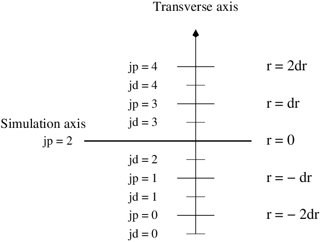
In Smilei, ghost cells in the radial direction are located “before” the axis. So if you have \(N_{ghost}\) ghost cells, you have as many primal points on the radial axis before reaching the actual geometric axis \(r=0\). If \(dr\) is a radial cell size, the dual radial axis is shifted by \(-dr/2\). Below is an example for \(N_{ghost}=2\). All equations in this section are given for this specific case. For different numbers of ghost cells, simply add the difference in all indices. \(jp\) and \(jd\) stand for the primal and dual indices.

Cancellation on axis

The first basic principle is that a mode 0 field defined on axis can only be longitudinal otherwise it would be ill defined. On the opposite, longitudinal fields on axis can only be of mode 0 since they do not depend on \(\theta\). From this we can already state that \(E_r^{m=0},\ E_t^{m=0},\ B_r^{m=0},\ B_t^{m=0},\ E_l^{m>0},\ B_l^{m>0}\) are zero on axis.

This condition is straight forward for primal fields in R which take a value on axis exactly. We simply set this value to zero.

\[ \begin{align}\begin{aligned}E_{\theta}^{m=0}[2] = 0\\B_r^{m=0}[2] = 0\\E_l^{m>0}[2] = 0\end{aligned}\end{align} \]

For dual fields in R, we set a value such as a linear interpolation between nearest grid points gives a zero on axis.

\[ \begin{align}\begin{aligned}E_r^{m=0}[2] = -E_r^{m=0}[3]\\B_{\theta}^{m=0}[2] = -B_{\theta}^{m=0}[3]\\B_l^{m>0}[2] = -B_l^{m>0}[3]\end{aligned}\end{align} \]

Transverse field on axis

The transverse electric field can be written as follows

\[\mathbf{E_\perp} = \mathbf{E_y} + \mathbf{E_z} = (E_r\cos{\theta}-E_{\theta}\sin{\theta})\mathbf{e_y} + (E_r\sin{\theta}+E_{\theta}\cos{\theta})\mathbf{e_z}\]

The transverse field on axis can not depend on \(\theta\) otherwise it would be ill defined. Therefore we have the following condition on axis:

\[\frac{\partial\mathbf{E_\perp}}{\partial\theta} = 0\ \forall\theta\]

which leads to the following relation:

\[\cos{\theta}\left(\frac{\partial E_r}{\partial\theta}-E_{\theta}\right) + \sin{\theta}\left(\frac{\partial E_{\theta}}{\partial\theta}+E_r\right)=0\ \forall\theta\]

Being true for all \(\theta\), this leads to

\[ \begin{align}\begin{aligned}\frac{\partial E_r}{\partial\theta}-E_{\theta}=0\ \forall\theta\\\frac{\partial E_{\theta}}{\partial\theta}+E_r=0\ \forall\theta\end{aligned}\end{align} \]

Remembering that for a given mode \(m\) and a given field \(F\), we have \(F=Re\left(\tilde{F}^m\exp{(-im\theta)}\right)\), we can write the previous equations for all modes \(m\) as follows:

(46)\[ \begin{align}\begin{aligned} \tilde{E_r}^m=\frac{i\tilde{E_{\theta}}^m}{m}\\ \tilde{E_r}^m=mi\tilde{E_{\theta}}^m\end{aligned}\end{align} \]

We have already established in the previuos section that the modes \(m=0\) must cancel on axis and we are concerned only about \(m>0\). Equations (46) can have a non zero solution only for \(m=1\) and is also valid for the magnetic field. We therefore conclude that all modes must cancel on axis except for \(m=1\).

\[ \begin{align}\begin{aligned}\tilde{E_{\theta}}^{m>1}[2] = 0\\\tilde{B_r}^{m>1}[2] = 0\\\tilde{E_r}^{m>1}[2] = -\tilde{E_r}^{m>1}[3]\\\tilde{B_{\theta}}^{m>1}[2] = -\tilde{B_{\theta}}^{m>1}[3]\end{aligned}\end{align} \]

Let’s now write the Gauss law for mode \(m=1\):

\[div(\mathbf{\tilde{E}^{m=1}})=\tilde{\rho}^{m=1}\]

where \(\rho\) is the charge density. We have already established that on axis the longitudinal field are zero for all modes \(m>0\). The charge density being a scalar field, it follows the same rule and is zero as well on axis. The continuity equation on axis and written in cylindrical coordinates becomes:

\[\frac{\tilde{E_r}^{m=1}-im\tilde{E_{\theta}}^{m=1}}{r} + \frac{\partial \tilde{E_r}^{m=1}}{\partial r} = 0\]

Eq. (46) already establishes that the first term is zero. It is only necessary to cancel the second term. To ensure this derivative cancels on axis we simply pick:

\[\tilde{E_r}^{m=1}[2] = \tilde{E}_r^{m=1}[3]\]

And equation (46) then gives

\[\tilde{E_{\theta}}^{m=1}(r=0) = -i\tilde{E_r}^{m=1}(r=0)\]

With a finite difference scheme, this is implemented as

\[\tilde{E_{\theta}}^{m=1}[2] = -\frac{i}{8}(9\tilde{E_r}^{m=1}[3]-\tilde{E_r}^{m=1}[4])\]

All the equation derived here are also valid for the magnetic field. But because of a different duality, it is more convenient to use a different approach. The equations (43) has a \(\frac{\tilde{E_l}}{r}\) term in the expression of \(B_r\) which makes it undefined on axis. Nevertheless, we need to evaluate this term for the mode \(m=1\) and it can be done as follows.

\[\lim_{r\to 0}\frac{E_l^{m=1}(r)}{r} = \lim_{r\to 0}\frac{E_l^{m=1}(r)-E_l^{m=1}(0)}{r}\]

since we established in the previous section that \(E_l^{m=1}(r=0)=0\). And by definition of a derivative we have:

\[\lim_{r\to 0}\frac{E_l^{m=1}(r)-E_l^{m=1}(0)}{r}=\frac{\partial E_l^{m=1} }{\partial r}(r=0)\]

This derivative can be evaluated by a simple finite difference scheme and using again that \(E_l^{m=1}\) is zero on axis we get:

(47)\[\lim_{r\to 0}\frac{E_l^{m=1}(r)}{r} = \frac{E_l^{m=1}(dr)}{dr}\]

Introducing this result in the standard FDTD scheme for \(B_r\) we get the axis bounday condition:

\[B_{r}^{m=1,n+1}[i,2] = B_{r}^{m=1,n}[i,2] + dt\left(\frac{i}{dr}E_l^{m=1}[i,3]+\frac{E_{\theta}^{m=1}[i+1,2]-E_{\theta}^{m=1}[i,2]}{dl}\right)\]

where the \(n\) indice indicates the time step and \(i\) the longitudinal indice. Exactly as for the electric field, we need to have \(B_{r}^{m=1}=iB_{\theta}^{m=1}\). With a similar interpolation we obtain the boundary condition on axis for \(B_{\theta}^{m=1}\):

\[B_{\theta}^{m=1}[2]=-2iB_{r}^{m=1}[2]-B_{\theta}^{m=1}[3]\]

Longitudinal field on axis

We have alreayd established that only modes \(m=0\) of longitudinal fields are non zero on axis. In order to get an evaluation of \(E_l^{m=0}\) on axis one can use the same approach as for \(B_r^{m=1}\). Since we have already shown that \(E_{\theta}^{m=0}\) is zero on axis, we have the following relation which is demonstrated using similar arguments as Eq. (47):

\[\lim_{r\to 0}\frac{1}{r}\frac{\partial rB_{\theta}^{m=0}}{\partial r} = \frac{4B_{\theta}^{m=0}(dr/2)}{dr}\]

Introducing this result in the standard FDTD expression of \(E_l\) we get:

\[E_{l}^{m=0,n+1}[i,2] = E_{l}^{m=0,n}[i,2] + dt\left(\frac{4}{dr}B_{\theta}^{m=0}[i,3]-J_{l}^{m=0}[i,2]\right)\]

Again, the \(n\) indice indicates the time step here.

Below axis

Fields “below” axis are primal fields data with indice \(j<2\) and dual fields with indice \(j<3\). These fields are not physical in the sense that they do not contribute to the reconstruction of any physical field in real space and are not obtained by solving Maxwell’s equations. Nevertheless, it is numerically convenient to give them a value in order to facilitate field interpolation for macro-particles near axis. This is already what is done for dual fields in \(r\) which cancel on axis for instance. We extend this logic to primal fields in \(r\) as well. For any given field \(F\), the symetric of \(F\) with respect to the axis is \(F\) if \(F\) is non zero on axis and \(-F\) if \(F\) is zero on axis:

\[ \begin{align}\begin{aligned}E_{l}^{m=0}[1] = E_{l}^{m=0}[3]\\E_{l}^{m>0}[1] = -E_{l}^{m>0}[3]\\E_{r}^{m\neq1}[2] = -E_{r}^{m\neq1}[3]\\E_{r}^{m=1}[2] = E_{r}^{m=1}[3]\\E_{\theta}^{m\neq1}[1] = -E_{\theta}^{m\neq1}[3]\\E_{\theta}^{m=1}[1] = E_{\theta}^{m=1}[3]\\B_{l}^{m=0}[2]=B_{l}^{m=0}[3]\\B_{l}^{m>0}[2]=-B_{l}^{m>0}[3]\\B_{r}^{m\neq1}[1] = -B_{r}^{m\neq1}[3]\\B_{r}^{m=1}[1] = B_{r}^{m=1}[3]\\B_{t}^{m\neq1}[2] = -B_{t}^{m\neq1}[3]\\B_{t}^{m=1}[2] = B_{t}^{m=1}[3]\end{aligned}\end{align} \]

Currents near axis

A specific treatment must be applied to charge and current densities near axis because the projector deposits charge and current “below” axis. Quantities below axis must be folded back onto their symetric “above” axis. Mode 0 contributions below axis are added to their “above axis” counterparts. On the opposite, strictly positive modes contributions are deduced. This ensures that a particle sitting on axis will have a net contribution to the domain only in mode 0 as expected because in that case \(\theta\) is not defined and therefore the deposition can not be a function of \(\theta\).

Using the continuity equation instead of Gauss law for transverse current of mode \(m=1\) on axis, we can derive the exact same boundary conditions on axis for current density as for the electric field.