
Laser propagation preprocessing
In Smilei, Lasers are provided as oscillating fields at the box boundaries.
For instance, at the xmin boundary of a 3D cartesian box, the user may define the
\(B_y(y,z,t)\) and \(B_z(y,z,t)\) profiles. But in some cases, the laser field
only known analytically at some arbitrary plane that does not coincide with the box
boundary. This appears typically in the case of tightly-focused beams that cannot be
described with a paraxial approximation.
At the beginning of the simulation (during the initialization), Smilei is able to perform a laser backwards propagation from an arbitrary plane to the box boundary. The calculated field is then injected from then boundary like a normal laser. From the user’s perspective, this simply requires the definition of the laser profile at some arbitrary plane.
The general technique is taken from [Thiele2016] but it has been improved for parallel computation in both 2D and 3D geometries. Further below, another improvement is presented: the propagation towards a tilted plane.
Theoretical background
The method employed for the propagation preprocessing is similar to the angular spectrum method. We illustrate this method on an arbitrary scalar field \(A\), but it is valid for all components of a field satisfying a wave equation:
\[c^2 \Delta A(x,y,z,t) = \partial_t^2 A(x,y,z,t)\]
The 3D Fourier transform of this equation for the variables \(y\), \(z\) and \(t\) gives:
\[(\partial_x^2 + k_x^2) \hat A(x,k_y,k_z,\omega) = 0\]
where \(k_y\), \(k_z\) and \(\omega\) are the conjugate variables in the frequency domain, and \(k_x(k_y,k_z,\omega) \equiv \sqrt{\omega^2/c^2-k_y^2-k_z^2}\). This equation has general solutions proportional to \(\exp(-i k_x x)\) for waves propagating towards positive \(x\). This means that, if the profile is known at some plane \(x=x_0+\delta\), the profile at \(x=x_0\) is obtained after multiplying \(\hat A\) by \(\exp(i k_x \delta)\):
\[\hat A(x_0,k_y,k_z,\omega) = \exp(i k_x \delta) \hat A(x_0+\delta,k_y,k_z,\omega)\]
To recover the field profile in real space, a 3D inverse Fourier transform would be sufficient. However, storing all values of the \((y,z,t)\) profile would consume too much time and disk space. Instead, Smilei does only a 2D inverse Fourier transform on \(k_y\) and \(k_z\). This results in a \(\tilde A(y,z,\omega)\) profile, where \(\omega\) are the temporal Fourier modes. Keeping only a few of these modes (the most intense ones) ensures a reasonable disk space usage.
The full \(A(y,z,t)\) profile is calculated during the actual PIC simulation, summing over the different \(\omega\).
Numerical process
Let us summarize how the calculation above is realized numerically. We suppose that the grid is 3D cartesian with the number of cells \((N_x, N_y, N_z)\) in the three directions, but the same process works in 2D. We write \(N_t\) the total number of timesteps.
The points 1 to 7 are realized during initialization.
1. The user profile \(B(y, z, t)\) is sampled
This profile corresponds to the magnetic field at the plane \(x=x_0+\delta\). Smilei calculates an array of size \((N_y, N_z, N_t)\) sampling this profile for all points of this plane, and all times of the simulation.
2. Smilei calculates the 3D Fourier transform along y, z and t
Using the FFT capabilities of the numpy python package, a parallel Fourier transform is achieved, giving a transformed array of the same size \((N_y, N_z, N_t)\). This array represents \(\hat B(k_y,k_z,\omega)\)
3. Frequencies with the most intense values are selected
Summing for all \(k_y\) and \(k_z\) provides a (temporal) spectrum of the wave. By default, the 100 frequencies giving the strongest values of this spectrum are kept, but this can be changed in the namelist (see
keep_n_strongest_modes). The resulting array is of size \((N_y, N_z, 100)\).
4. The array is multiplied by the propagation term
This term \(\exp(i k_x \delta)\) depends on the coordinates of the array because \(k_x\) is a function of \(k_y\), \(k_z\) and \(\omega\). Note that the \(\delta\) corresponds to the attribute
offset.
5. The inverse 2D Fourier transform is computed
This provides an array representing \(\tilde B(y,z,\omega)\)
6. The array is stored in an HDF5 file
This file is named
LaserOffset0.h5,LaserOffset1.h5, etc. if there are several lasers.
7. Each patch reads the part of the array that it owns
This means that each patch of the PIC mesh will own a distinct portion of the overall array.
The point 8 is realized at runtime, for each iteration.
8. For each timestep, the laser profile is calculated
The 100 selected modes are summed according to
\[B(y,z,t) = f(y,z,t) \sum_\omega \left| \tilde B(y,z,\omega) \right| \sin\left(\omega t + \phi(y,z,\omega)\right)\]where \(\phi\) is the complex argument of \(\tilde B\) and \(f(y,z,t)\) is an additional
extra_envelope, defined by the user. This envelope helps removing spurious repetitions of the laser pulse that can occur due to the limited number of frequencies that are kept.
Tilted plane
The method above describes a wave propagation between two parallel planes. In Smilei, a technique inspired from [Matsushima2003] allows for the propagation from a title plane.
This rotation happens in the Fourier space: wave vectors \(k_x\) and \(k_y\) are rotated around \(k_z\) by an angle \(\theta\), according to
This transforms \(\hat A(x,k_y,k_z,\omega)\) into \(\hat A^\prime(x,k_y^\prime,k_z,\omega)\), thus the operation is merely a change of one variable (\(k_y\)).
Numerically, the process is not that straightforward because \(\hat A^\prime\) is an array in which the axis \(k_y^\prime\) is linearly sampled, but the corresponding values \(k_y\) do not match this linear sampling. We developed an interpolation method to obtain the transformed values at any point.
In the end, the prescribed laser profile lies in a plane located at a distance \(\delta\) and rotated around \(z\) by an angle \(\theta\), according to the following figure.
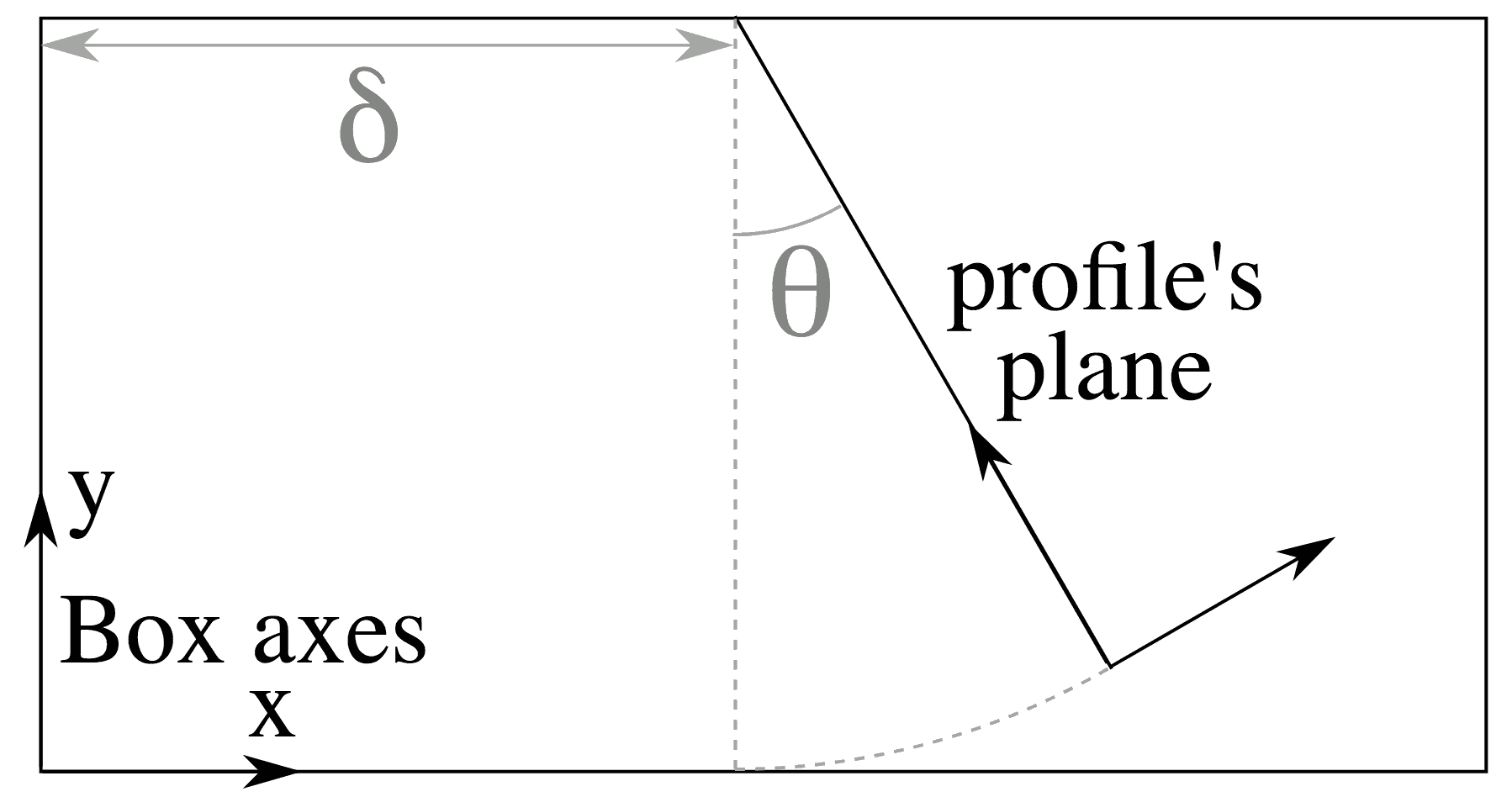
Fig. 63 The position of the plane where the laser profile is defined, with respect to the box.