
Generation of the external tables
By default, Smilei embeds tables directly in the sources. Nonetheless, a user may want to use different tables. For this reason, Smilei can read external tables.
Several physical mechanisms can use external tables to work:
Radiation loss and photon emission via nonlinear inverse Compton scattering (see High-energy photon emission & radiation reaction)
Electron-positon pair creation via the Multiphoton Breit-Wheeler (see Multiphoton Breit-Wheeler pair creation)
An external tool called smilei_tables is available to generate these tables.
Installation
The C++ sources of this tool is located in tools/tables.
Required dependencies are the following:
A C++11 compiler
A MPI library
HDF5 installed at least in serial
Boost is a C++ library that provides efficient advanced mathematical functions.
This is the only dependency not required to install Smilei.
This library can be easily installed manually on Linux, MacOS or Windows systems.
It is also available via different package managers (Debian, Homebrew).
The environment variable BOOST_ROOT must be defined.
The tool can be then installed using the makefile and the argument tables:
make tables
The compilation generates an executable called smilei_tables on the root of the repository.
Execution
The tool works with command line arguments. For each physical mechanism, smilei_tables generates all the tables for this mechanism. The first argument therefore corresponds to the physical mechanism:
Nonlinear inverse Compton scattering:
nicsMultiphoton Breit-Wheeler:
mbwFor help:
-hor`--help
mpirun -np <number of processes> ./smilei_tables -h
Then, once the physical mechanism is selected, the following arguments are the numerical parameters for the table generation.
For each physical argument, -h or --help gives the full list of arguments.
For Nonlinear inverse Compton Scattering:
mpirun -np <number of processes> ./smilei_tables nics -h

_______________________________________________________________________

Smilei Tables
_______________________________________________________________________

You have selected the creation of tables for the nonlinear inverse Compton scattering.

Help page specific to the nonlinear inverse Compton Scattering:

List of available commands:
-h, --help                       print a help message and exit.
-s, --size       int int         respective size of the particle and photon chi axis. (default 128 128)
-b, --boundaries double double   min and max of the particle chi axis. (default 1e-3 1e3)
-e, --error      int             compute error due to discretization and use the provided int as a number of draws. (default 0)
-t, --threshold  double          Minimum targeted value of xi in the computation the minimum particle quantum parameter. (default 1e-3)
-p, --power      int             Maximum decrease in order of magnitude for the search for the minimum particle quantum parameter. (default 4)
-v, --verbose                    Dump the tables
For multiphoton Breit-Wheeler:
mpirun -np <number of processes> ./smilei_tables mbw -h

_______________________________________________________________________

Smilei Tables
_______________________________________________________________________

You have selected the creation of tables for the multiphoton Breit Wheeler process.

Help page specific to the multiphoton Breit-Wheeler:

List of available commands:
-h, --help                       print a help message and exit.
-s, --size       int int         respective size of the photon and particle chi axis. (default 128 128)
-b, --boundaries double double   min and max of the photon chi axis. (default 1e-2 1e2)
-e, --error      int             compute error due to discretization and use the provided int as a number of draws. (default 0)
-t, --threshold  double          Minimum targeted value of xi in the computation the minimum photon quantum parameter. (default 1e-3)
-p, --power      int             Maximum decrease in order of magnitude for the search for the minimum photon quantum parameter. (default 4)
-v, --verbose                    Dump the tables
The tables are generated where the code is executed using HDF5 with the following names:
Nonlinear inverse Compton Scattering:
radiation_tables.h5multiphoton Breit-Wheeler:
multiphoton_breit_wheeler_tables.h5
Precomputed tables
We have computed some tables with several levels of discretization that you can download here.
256 points
This table size is a good compromise between accuracy and memory cost. 2D tables can fit in L2 cache although the pressure on the cache will be high. This set of tables is the one included by default in the sources of Smilei
mpirun -np <number of processes> ./smilei_tables nics -s 256 256 -b 1e-4 1e3
tables_256/radiation_tables.h5
mpirun -np <number of processes> ./smilei_tables mbw -s 256 256 -b 1e-2 1e2
tables_256/multiphoton_breit_wheeler_tables.h5
These tables can be generated on a normal desktop computer in few minutes.
512 points
With a size of 512 points in 1D and 512x512 for 2D tables, these tables offer better accuracy at a larger memory cost. 2D tables of this size are too large to fit in L2 cache but can be contained in L3.
mpirun -np <number of processes> ./smilei_tables nics -s 512 512 -b 1e-4 1e3
tables_512/radiation_tables.h5
mpirun -np <number of processes> ./smilei_tables mbw -s 512 512 -b 1e-2 1e2
1024 points
With a size of 1024 points in 1D and 1024x1024 for 2D tables, these tables offer the best accuracy at a high memory cost (around 8.5 Mb per file). 2D tables of this size are too large to fit in L2 cache and L3 cache.
mpirun -np <number of processes> ./smilei_tables nics -s 1024 1024 -b 1e-4 1e3
tables_1024/radiation_tables.h5
mpirun -np <number of processes> ./smilei_tables mbw -s 1024 1024 -b 1e-2 1e2
Python visualization scripts
You can easily visualize the tables provided by our tools using the python scripts located in the tools/tables folder:
show_nonlinear_inverse_Compton_scattering.pyshow_multiphoton_Breit_Wheeler.py
For instance:
python ./tools/tables/show_nonlinear_inverse_Compton_scattering.py ./radiation_tables.h5
Detailed description of the tables
Nonlinear Inverse Compton Scattering
The file radiation_tables.h5 is used for the nonlinear inverse Compton scattering radiation
mechanism described in the dedicated section.
It first contains the integfochi table that represents
the integration of the synchortron emissivity of Ritus et al:
where
The \(x\) value corresponds to the photon quantum parameter. We integrate the whole spectrum. This table is used by the Monte-Carlo method to compute the radiation emission cross-section.
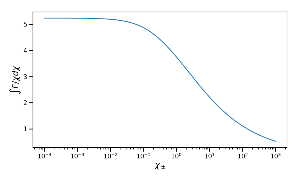
Fig. 64 Plot of the integfochi table for a particle quantum parameter ranging from \(\chi = 10^{-4}\) to \(10^{3}\) using the pre-computed table of 512 points.
The table h is used for the Niel stochastic model ([Niel2018a]).
It is given by the following integration:
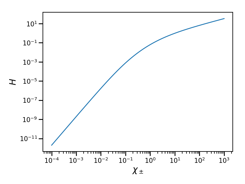
Fig. 65 Plot of the h table for a particle quantum parameter ranging from \(\chi = 10^{-4}\) to \(10^{3}\) using the pre-computed table of 512 points.
The table min_photon_chi_for_xi is the minimum boundary used
by the table xi for the photon quantum parameter axis.
This minimum value \(\chi_{\gamma,\min}\) is computed using the following inequality:
We generally use \(\varepsilon = 10^{-3}\).
It corresponds to the argument parameter xi_threshold.
We have to determine a minimum photon quantum parameter because
we cannot have a logarithmic discretization starting from 0.
It basically means that we ignore the radiated energy below \(\chi_{\gamma,\min}\)
that is less than \(10^{-3}\) of the total radiated energy.
The parameter xi_power is the precision of the \(\chi_{\gamma,\min}\) value.
For instance, a xi_power of 4 as used for our tables mean that we look for a precision of 4 digits.
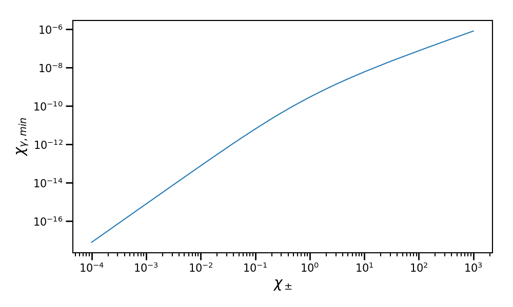
Fig. 66 Plot of the minimal photon quantum parameter \(\chi_{\gamma,\min}\)
corresponding to the minimum boundary of the xi table
as a function of the particle quantum parameter \(\chi_\pm\) ranging
from \(10^{-4}\) to \(10^{3}\). It corresponds to the pre-computed table of 512 points.
The table xi corresponds to the following fraction:
For a given \(\chi_\pm\) and a randomly drawn parameter \(\xi\), we obtain the quantum parameter \(\chi_\gamma\) of the emitted photon. This method is used by the Monte-Carlo method to determine the radiated energy of the emitted photon. For a given \(\chi_\pm\), \(\chi_\gamma\) ranges from \(\chi_{\gamma,\min}\) to \(\chi_\pm\).
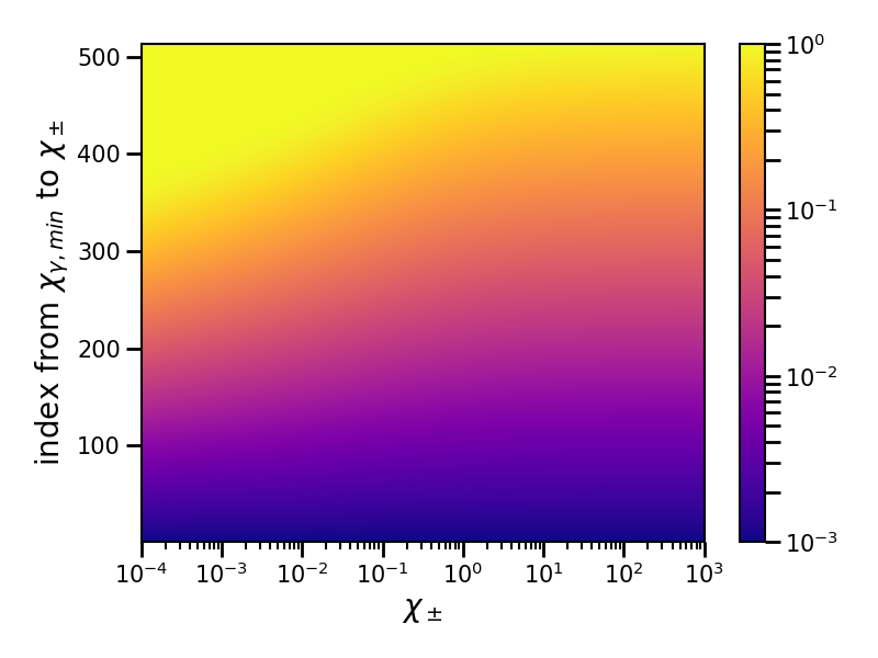
Fig. 67 Plot of the xi table as a function of the particle quantum parameter \(\chi_\pm\) and index for the \(\chi_\gamma\) axis. The \(\chi_\pm\) axis ranges from \(10^{-4}\) to \(10^{3}\). The \(\chi_\gamma\) axis ranges from \(\chi_{\gamma,\min}\) to \(\chi_\pm\). It corresponds to the pre-computed table of 512 points.
Multiphoton Breit-Wheeler
The file multiphoton_breit_wheeler_tables.h5 is used for the multiphoton Breit-Wheeler process
described in the dedicated section.
It first contains the T table that represents
the following integration:
where
And
It is used to compute the production rate of electron-positron pairs from a single photon of quantum parameter \(\chi_\gamma\). In the Monte-Carlo algorithm, it is used to determine the photon decay probability.
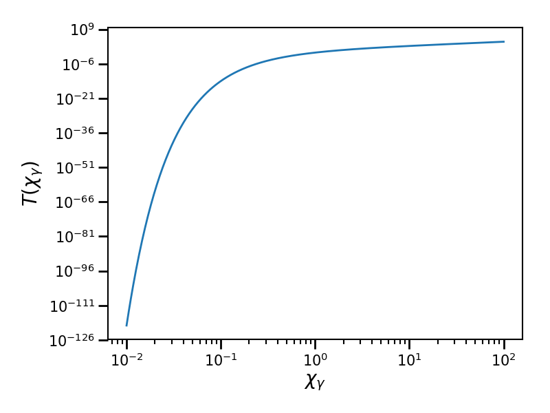
Fig. 68 Plot of the table T
as a function of the photon quantum parameter \(\chi_\gamma\) ranging
from \(10^{-2}\) to \(10^{2}\).
It corresponds to the pre-computed table size of 512 points.
The table min_particle_chi_for_xi is the minimum boundary used
by the table xi for the particle quantum parameter axis.
The particle can be either a positron or an electron.
The mechanism is symmetric.
This minimum value \(\chi_{\pm,\min}\) is computed using the following inequality:
We use here \(\varepsilon = 10^{-9}\).
It corresponds to the argument parameter xi_threshold.
We have to determine a minimum photon quantum parameter because
we cannot have a logarithmic discretization starting from 0.
The parameter xi_power is the precision of the \(\chi_{\pm,\min}\) value.
For instance, a xi_power of 4 as used for our tables mean that we look for a precision of 4 digits.
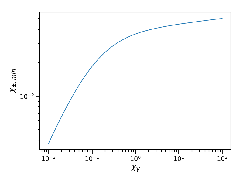
Fig. 69 Plot of the minimal particle quantum parameter \(\chi_{\pm,\min}\) corresponding to the minimum boundary of the xi table as a function of the photon quantum parameter \(\chi_\gamma\) ranging from \(10^{-2}\) to \(10^{2}\). It corresponds to the pre-computed table of 512 points.
The table xi corresponds to the following fraction:
For a given \(\chi_\gamma\) and a randomly drawn parameter \(\xi\), we obtain the quantum parameter \(\chi_\pm\) of either the generated electron or positron. Once we have one, we deduce the second from \(\chi_\gamma = \chi_+ + \chi_-\) This method is used by the Monte-Carlo method to determine the energy of the created electron and the positron. For a given \(\chi_\gamma\), \(\chi_\pm\) ranges from \(\chi_{\pm,\min}\) to \(\chi_\gamma\).
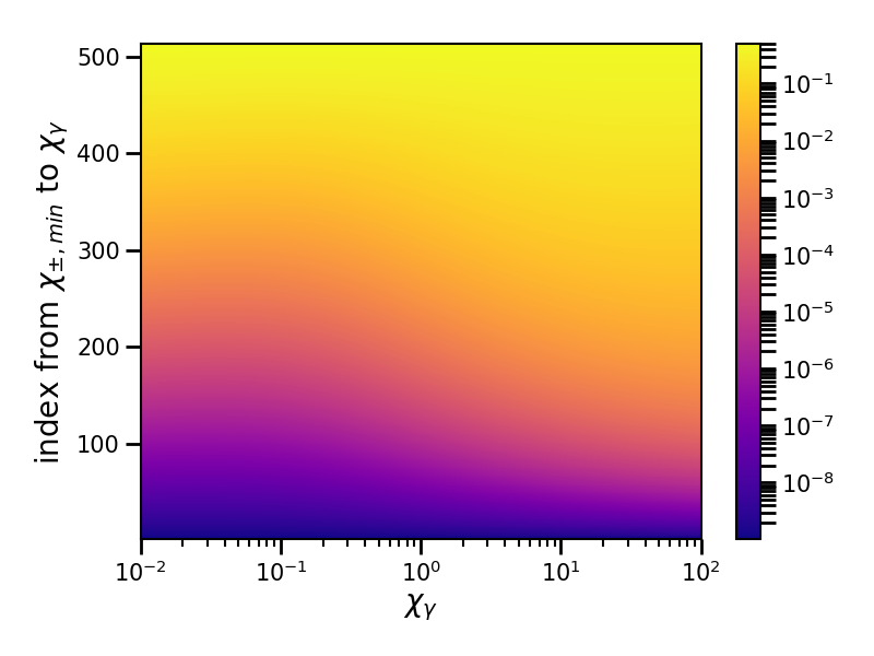
Fig. 70 Plot of the xi table as a function of the photon quantum parameter \(\chi_\gamma\) and index for the \(\chi_\pm\) axis. The \(\chi_\gamma\) axis ranges from \(10^{-2}\) to \(10^{2}\). The \(\chi_\pm\) axis ranges from \(\chi_{\pm,\min}\) to \(\chi_\pm\). It corresponds to the pre-computed table of 512 points.