
Ionization
Four types of ionization have been introduced in Smilei: collisional ionization, field ionization, envelope ionization (time average field) or custom ionization using user defined rates.
Collisional ionization
Ionization may occur during collisions. A detailed description is given on the corresponding page.
Field ionization
Field ionization is a process of particular importance for laser-plasma interaction in the ultra-high intensity regime. It can affect ion acceleration driven by irradiating a solid target with an ultra-intense laser, or can be used to inject electrons through the accelerating field in laser wakefield acceleration. This process is not described in the standard PIC (Vlasov-Maxwell) formulation, and an ad hoc description needs to be implemented. A Monte-Carlo module for field ionization has thus been developed in Smilei, closely following the method proposed in [Nuter2011].
Physical model for field ionization
This scheme relies on the quasi-static rate for tunnel ionization derived in [Perelomov1966], [Perelomov1967] and [Ammosov1986]. Considering an ion with atomic number \(Z\) being ionized from charge state \(Z^\star-1\) to \(Z^\star \le Z\) in a constant electric field \(\mathbf{E}\) of magnitude \(\vert E\vert\), the ionization rate reads:
where \(I_p\) is the \(Z^{\star}-1\) ionization potential of the ion, \(n^\star=Z^\star/\sqrt{2 I_p}\) and \(l^\star=n^\star-1\) denote the effective principal quantum number and angular momentum, and \(l\) and \(m\) denote the angular momentum and its projection on the laser polarization direction, respectively. \(\Gamma_{\rm ADK, DC}\), \(I_p\) and \(E\) are here expressed in atomic units The coefficients \(A_{n^\star,l^\star}\) and \(B_{l,\vert m\vert}\) are given by:
where \(\Gamma(x)\) is the gamma function. Note that considering an electric field \(E=\vert E\vert\,\cos(\omega t)\) oscillating in time at the frequency \(\omega\), averaging Eq. (9) over a period \(2\pi/\omega\) leads to the well-known cycle-averaged ionization rate:
We note that the initial velocity of the electrons newly created by ionization is chosen as equal to the ion velocity. This constitutes a minor violation of momentum conservation, as the ion mass is not decreased after ionization.
In Smilei, two models are available to compute the ionization rate of (9).
PPT-ADK modelIn the classical model, the ionization rate of (9) is computed for \(\vert m \vert=0\) only. Indeed, as shown in [Ammosov1986], the ratio \(R\) of the ionization rate computed for \(\vert m\vert=0\) by the rate computed for \(\vert m\vert=1\) is:
\[R = \frac{\Gamma_{{\rm qs},\vert m \vert = 0}}{\Gamma_{{\rm qs},\vert m \vert = 1}} = 2\frac{(2\,I_p)^{3/2}}{\vert E\vert} \simeq 7.91\,10^{-3} \,\,\frac{(I_p[\rm eV])^{3/2}}{a_0\,\hbar\omega_0[\rm eV]}\,,\]where, in the practical units formulation, we have considered ionization by a laser with normalized vector potential \(a_0=e\vert E\vert /(m_e c \omega_0)\), and photon energy \(\hbar\omega_0\) in eV. Typically, ionization by a laser with wavelength \(1~{\rm \mu m}\) (correspondingly \(\hbar \omega_0 \sim 1~{\rm eV}\)) occurs for values of \(a_0\ll 1\) (even for large laser intensities for which ionization would occur during the rising time of the pulse) while the ionization potential ranges from a couple of eV (for electrons on the most external shells) up to a few tens of thousands of eV (for electrons on the internal shell of high-Z atoms). As a consequence, \(R\gg1\), and the probability of ionization of an electron with magnetic quantum number \(\vert m \vert=0\) greatly exceeds that of an electron with \(\vert m \vert = 1\).
PPT-ADK model with account for\(m\neq 0\) experimentalIn this model, first implemented in [Mironov2025], dependence on the magnetic quantum number \(m\) is added.
\(m\) is attributed to each electron in accordance with the following rules:
1. Since \(\Gamma_z(m=0)>\Gamma_z(m=1)>\Gamma_z(m=2)>...\) we assume that for electrons with the same azimuthal quantum number \(l\), the states with the lowest value of \(|m|\) are ionized first.
2. Electrons with the same azimuthal quantum number \(l\) occupy the sub-shells in the order of increasing \(|m|\) and for the same \(|m|\) in the order of increasing \(m\).
With this algorithm, by knowing the atomic number A, we can assign a unique set of quantum numbers \(nlm\) to each electron on the atomic sub-shells and identify their extraction order during successive ionization. The ionization rate also accounts for multiple electrons having the same energy levels via the degeneracy factor.
Warning
Although this model uses less assumptions than the PPT-ADK model, [Mironov2025] shows that these corrections introduce a dependency on the ionization path chosen for the atom and may actually lead to less accurate results than the default ADK model. A non-sequential ionization path is necessary for this model to be accurate and will be proposed in a later version of the code hence the experimental tag. A reference implementation of non-sequential ionization is provided in [Mironov2025].
Barrier Suppression Ionization
When the electric field applied on a bound electron is greater than a certain threshold, that electron is able to classically escape from the atom, without tunneling through the potential barrier. To properly describe the ionisation rates in these regimes, and the transition regime from tunneling to barrier suppression, Smilei implements two ways to extend the tunneling ionization rate to the barrier-suppression regime.
Tong & Lin
The formula proposed by Tong and Lin [Tong2005] extends the tunneling ionization rate to the barrier-suppression regime. This is achieved by introducing an empirical factor in (9):
\[\Gamma_{Z^\star}^{TL} = \Gamma_{Z^\star} \times \exp \left(-\alpha_{TL}n^{\star2}\frac{E}{(2I_p)^{3/2}}\right),\]where \(\alpha_{TL}\) is an emprirical constant with value typically from 6 to 9. The actual value should be guessed from empirical data. When such data is not available, the formula can be used for qualitative analysis of the barrier-suppression ionization (BSI), e.g. see [Ciappina2020]. The module was tested to reproduce the results from this paper.
Kostyukov Artemenko Golovanov
This is a piecewise function, first proposed by Kostyukov, Artemenko and Golovanov (KAG) in [Artemenko2017] and [Kostyukov2018], and published in [Ouatu2022] as follows:
\[\begin{split}\Gamma_{KAG} = \begin{cases} \Gamma_{qs,|m|=0}, & E < E_1 \\ \Gamma_{BM}, & E_1 < E < E_2 \\ \Gamma_{BSI}, & E > E_2 \end{cases}\end{split}\]where \(\Gamma_{BM} = 2.4 E^2 (I_H/I_p)^2\) is the rate in the transition regime between the tunnel and barrier suppression ionisation regimes [Bauer1999] and \(\Gamma_{BSI} = 0.8 E \sqrt{I_H/I_p}\) is the barrier suppression ionisation rate [Artemenko2017], \(E_1\) and \(E_2\) are the intersection points of \(\Gamma_{ADK}\) with \(\Gamma_{BM}\) and \(\Gamma_{BM}\) with \(\Gamma_{BSI}\) respectively, such that the function is continuous, and \(I_H\) is the ionisation potential of hydrogen.
Monte-Carlo scheme
In Smilei, tunnel ionization is treated for each species (defined by the user as subject to field ionization) right after field interpolation and before applying the pusher. For all quasi-particles (henceforth referred to as quasi-ion) of the considered species, a Monte-Carlo procedure has been implemented that allows to treat multiple ionization events in a single timestep. It relies on the cumulative probability derived in Ref. [Nuter2011]:
to ionize from 0 to \(k\) times a quasi-ion with initial charge state \(Z^{\star}-1\) during a simulation timestep \(\Delta t\), \(p_j^{Z^{\star}-1}\) being the probability to ionize exactly \(j\) times this ion.
The Monte-Carlo procedure proceeds as follows. A random number \(r\) with uniform distribution between 0 and 1 is picked. If \(r\) is smaller than the probability \(p_0^{Z^{\star}-1}\) to not ionize the quasi-ion, then the quasi-ion is not ionized during this time step. Otherwise, we loop over the number of ionization events \(k\), from \(k=1\) to \(k_{\rm max}=Z-Z^{\star}+1\) (for which \(F_{k_{\rm max}}^{Z^{\star}-1}=1\) by construction), until \(r<F_k^{Z^{\star}-1}\). At that point, \(k\) is the number of ionization events for the quasi-ion. A quasi-electron is created with the numerical weight equal to \(k\) times that of the quasi-ion, and with the same velocity as this quasi-ion. The quasi-ion charge is also increased by \(k\).
Finally, to ensure energy conservation, an ionization current \({\bf J}_{\rm ion}\) is projected onto the simulation grid such that
Benchmarks
In what follows, we present two benchmarks of the field ionization model. Both benchmarks consist in irradiating a thin (one cell long) neutral material (hydrogen or carbon) with a short (few optical-cycle long) laser with wavelength \(\lambda_0 = 0.8~{\mu m}\).
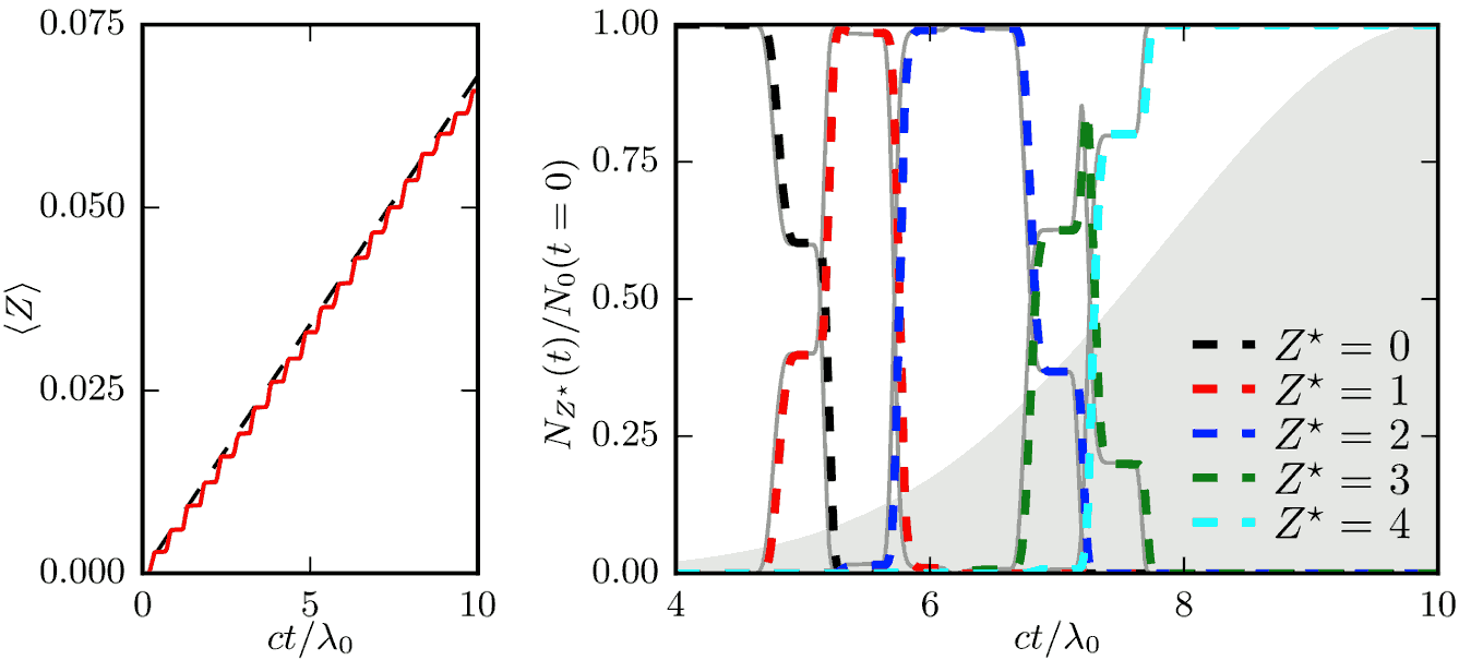
Fig. 27 Results of two benchmarks for the field ionization Model. Top: Average charge state of hydrogen ions as a function of time when irradiated by a laser. The red solid line corresponds to PIC results, the dashed line corresponds to theoretical predictions using the cycle-averaged ADK growth rate of (10). Bottom: Relative distribution of carbon ions for different charge states as a function of time. Dashed lines correspond to PIC results, thin gray lines correspond to theoretical predictions obtained from (12). The Gaussian gray shape indicates the laser electric field envelope.
In the first benchmark, featuring hydrogen, the laser intensity is kept constant at \(I_L = 10^{14}~{\rm W/cm^2}\), corresponding to a normalized vector potential \(a_0 \simeq 6.81 \times 10^{-3}\), over 10 optical cycles. The resulting averaged ion charge in the simulation is presented as a function of time in Fig. 27 (left). It is found to be in excellent agreement with the theoretical prediction considering the cycle averaged ionization rate \(\Gamma_{\rm ADK} \simeq 2.55\times10^{12}~{\rm s^{-1}}\) computed from (10).
The second benchmark features carbon ions. The laser has a peak intensity \(I_L = 5 \times 10^{16}~{\rm W/cm^2}\), corresponding to a normalized vector potential \(a_0 \simeq 1.52 \times 10^{-1}\), and a gaussian time profile with FWHM \(\tau_L=5~\lambda_0/c\) (in terms of electric field). Fig. 27 (right) shows, as function of time, the relative distribution of carbon ions for different charge states (from 0 to \(+4\)). These numerical results are shown to be in excellent agreement with theoretical predictions obtained by numerically solving the coupled rate equations on the population \(N_i\) of each level \(i\):
with \(\delta_{i,j}\) the Kroenecker delta, and \(\Gamma_i\) the ionization rate of level \(i\). Note also that, for this configuration, \(\Delta t \simeq 0.04~{\rm fs}\) is about ten times larger than the characteristic time \(\Gamma_{\rm ADK}^{-1} \simeq 0.006~{\rm fs}\) to ionize \({\rm C}^{2+}\) and \({\rm C}^{3+}\) so that multiple ionization from \({\rm C}^{2+}\) to \({\rm C}^{4+}\) during a single timestep does occur and is found to be correctly accounted for in our simulations.
Field ionization with a laser envelope
In a typical PIC simulation, the laser oscillation is sampled frequently in time, thus the electric field can be considered static within a single timestep where ionization takes place, and the ionization rate in DC, i.e. \(\Gamma_{\rm ADK, DC}\) from Eq. (9) can be used at each timestep. Furthermore, if the atom/ion from which the electrons are stripped through ionization is at rest, for momentum conservation the new electrons can be initialized with zero momentum. If a laser ionized the atom/ion, the new electrons momenta will quickly change due to the Lorentz force.
Instead, in presence of a laser envelope (see Laser envelope model) an ad hoc treatment of the ionization process averaged over the scales of the optical cycle is necessary, since the integration timestep is much greater than the one used in those typical PIC simulations [Chen2013]. Thus, in this case a ionization rate \(\Gamma_{\rm ADK, AC}\) obtained averaging \(\Gamma_{\rm ADK, DC}\) over the laser oscillations should be used at each timestep to have a better agreement with a correspondent standard laser simulation. Afterwards, the momentum of the newly created electrons must be properly initialized taking into account of the averaging process in the definition of the particle-envelope interaction.
For circular polarization, i.e. ellipticity = 1,
\(\Gamma_{\rm ADK, AC}=\Gamma_{\rm ADK, DC}\), since the field does not change
its magnitude over the laser oscillations.
For linear polarization, i.e. ellipticity = 0 :
Normally the laser is intense enough to be the main cause of ionization, but to take into account possible high total fields \(E\) not described only by an envelope, in Smilei a combination \(E=\sqrt{\vert E_{plasma}\vert^{2}+\vert\tilde{E}_{envelope}\vert^{2}}\) is used instead of \(E\) in the above formulas. The field \(\tilde{E}_{plasma}\) represents the (low frequency) electric field of the plasma, while \(\vert\tilde{E}_{envelope} \vert=\sqrt{\vert\tilde{E}\vert^2+\vert\tilde{E}_x\vert^2}\) takes into account the envelopes of both the transverse and longitudinal components of the laser electric field (see Laser envelope model for details on their calculation).
After an electron is created through envelope tunnel ionization, its initial transverse momentum \(p_{\perp}\) is assigned as described in [Tomassini2017]. For circular polarization, in the case of an electron subject to a laser transverse envelope vector potential \(\tilde{A}\), the magnitude of its initial transverse momentum is set as \(\vert p_{\perp}\vert = \vert\tilde{A}\vert\) and its transverse direction is chosen randomly between \(0\) and \(2\pi\). For linear polarization, the initial transverse momentum along the polarization direction is drawn from a gaussian distribution with rms width \(\sigma_{p_{\perp}} = \Delta\vert\tilde{A}\vert\), to reproduce the residual rms transverse momentum spread of electrons stripped from atoms by a linearly polarized laser [Schroeder2014]. The parameter \(\Delta\) is defined as [Schroeder2014]:
This approximation is valid for regimes where \(\Delta\ll 1\). Additionally, in Smilei the initial longitudinal momentum of the new electrons is initialized, to recreate the statistical features of the momentum distribution of the electrons created through ionization. An electron initially at rest in a plane wave with vector potential of amplitude \(\vert\tilde{A}\vert\) propagating along the positive \(x\) direction is subject to a drift in the wave propagation direction [Gibbon]. An electron stripped from an atom/ion through envelope ionization by a laser can be approximated locally as in a plane wave, thus averaging over the laser oscillations yields a positive momentum in the \(x\) direction. Thus, each electron created from envelope tunnel ionization is initialized with \(p_x = \vert\tilde{A}\vert^2/4+\vert p_{\perp}\vert^2/2\) for linear polarization, where \(p_{\perp}\) is drawn as described above. For circular polarization, each of these electron is initalized with \(p_x = \vert\tilde{A}\vert^2/2\). This technique allows to take into account the longitudinal effects of the wave on the initial momentum, that start to be significant when \(\vert\tilde{A}\vert>1\), effects which manifest mainly as an initial average longitudinal momentum. For relativistic regimes, the longitudinal momentum effects significantly change the relativistic Lorentz factor and thus start to significantly influence also the evolution of the transverse momenta.
If the envelope approximation hypotheses are satisfied, the charge created with ionization and the momentum distribution of the newly created electrons computed with this procedure should agree with those obtained with a standard laser simulation, provided that the comparison is made after the end of the interaction with the laser. Examples of these comparisons and the derivation of the described electron momentum initialization can be found in [Massimo2020a]. A comparison made in a timestep where the interaction with the laser is still taking place would show the effects of the quiver motion in the electron momenta in the standard laser simulation (e.g. peaks in the transverse momentum spectrum). These effects would be absent in the envelope simulation.
Apart from the different ionization rate and the ad hoc momentum initialization of the new electrons, the implementation of the field ionization with a laser envelope follows the same procedure described in the above section treating the usual field ionization.
In presence of a laser envelope, an energy conservation equation analogous to (11) cannot be written, since the information about the direction of the ionizing field is lost with the envelope description. However, in many situations where the envelope approximation is valid the ion current can be neglected and the error on energy conservation is negligible.
User-defined ionization rate
Smilei can treat ionization considering a fixed rate prescribed by the user.
The ionization rates are defined, for a given Species, as described here.
The Monte-Carlo procedure behind the treatment of ionization in this case closely follows
that developed for field ionization.
Warning
Note that, in the case of a user-defined ionization rate, only single ionization event per timestep are possible.
Let us introduce two benchmarks for which the rate of ionization is defined by the user. The first benchmark considers an initially neutral species that can be potentially ionized twice. To run this case, a constant and uniform ionization rate is considered that depends only on the particle current charge state. For this particular case, we have considered a rate \(r_0 = 0.1\) (in code units) for ionization from charge state 0 to 1, and a rate \(r_1 = 0.05\) (in code units) for ionization from charge state 1 to 2. The simulation results presented in Fig. Fig. 28 (top panel) shows the time evolution of the fraction in each possible charge states (\(Z=0\), \(Z=1\) and \(Z=2\)). Super-imposed (dashed lines) are the corresponding theoretical predictions.
The second benchmark features an initially neutral species homogeneously distributed in the simulation box. The ionization rate is here chosen as a function of the spatial coordinate \(x\), and reads \(r(x) = r_0 \exp(-(x-x_c)^2/2)\) with \(r_0 = 0.02\) the maximum ionization rate and \(x_c=5\) the center of the simulation box. The simulation results presented in Fig. Fig. 28 (bottom panel) shows, at the end of the simulation \(t=20\), the electron number density as a function of space. Super-imposed (in red) is the corresponding theoretical prediction.
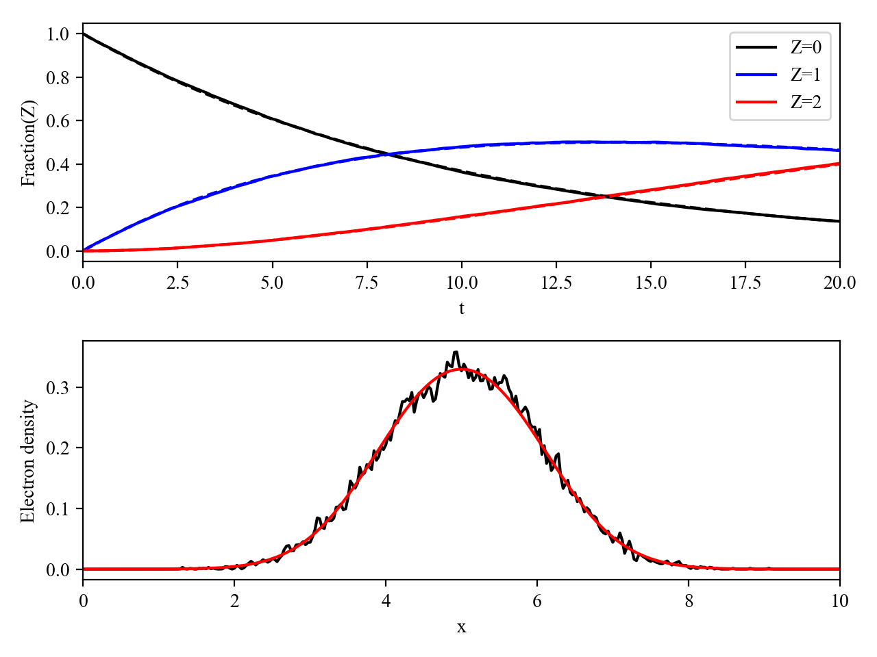
Fig. 28 Results of the two benchmarks for the ionization model using user-defined rates as described above.