High-energy photon emission & radiation reaction

Accelerated charges emit electromagnetic radiation, and by doing so, lose some of their energy and momentum. This process is particularly important for high-energy particles traveling in strong electromagnetic fields where it can strongly influence the dynamics of the radiating charges, a process known as radiation reaction.

In Smilei, different modules treating high-energy photon emission & its back-reaction have been implemented. We first give a short overview of the physics (and assumptions) underlying these modules, before giving more pratical information on what each module does. We then give examples & benchmarks, while the last two sections give additional information on the implementation of the various modules and their performances.

Warning

The processes discussed in this section bring into play a characteristic length [the classical radius of the electron \(r_e = e^2/(4\pi \epsilon_0 m_e c^2)\) in classical electrodynamics (CED) or the standard Compton wavelength \(\lambda_C=\hbar/(m_e c)\) in quantum electrodynamics (QED)]. As a result, a simulation will require the user to define the absolute scale of the system by defining the reference_angular_frequency_SI parameter (see Units for more details).

Also note that, unless specified otherwise, SI units are used throughout this section, and we use standard notations with \(m_e\), \(e\), \(c\) and \(\hbar\) the electron mass, elementary charge, speed of light and reduced Planck constant, respectively, and \(\epsilon_0\) the permittivity of vacuum.

---

Inverse Compton scattering

This paragraph describes the physical model and assumptions behind the different modules for high-energy photon emission & radiation reaction that have been implemented in Smilei. The presentation is based on the work [Niel2018a].

Assumptions

All the modules developed so far in Smilei assume that:

• the radiating particles (either electrons or positrons) are ultra-relativistic (their Lorentz factor \(\gamma \gg 1\)), hence radiation is emitted in the direction given by the radiating particle velocity,

• the electromagnetic field varies slowly over the formation time of the emitted photon, which requires relativistic field strengths [i.e., the field vector potential is \(e\vert A^{\mu}\vert/(mc^2) \gg 1\)], and allows to use quasi-static models for high-energy photon emission (locally-constant cross-field approximation),

• the electromagnetic fields are small with respect to the critical field of Quantum Electrodynamics (QED), more precisely both field invariants \(\sqrt{c^2{\bf B}^2-{\bf E}^2}\) and \(\sqrt{c{\bf B}\cdot{\bf E}}\) are small with respect to the Schwinger field \(E_s = m^2 c^3 / (\hbar e) \simeq 1.3 \times 10^{18}\ \mathrm{V/m}\),

• all (real) particles radiate independently of their neighbors (incoherent emission), which requires the emitted radiation wavelength to be much shorter than the typical distance between (real) particles \(\propto n_e^{-1/3}\).

Rate of photon emission and associated quantities

Under these assumptions, high-energy photon emission reduces to the incoherent process of nonlinear inverse Compton scattering. The corresponding rate of high-energy photon emission is given by [Ritus1985]:

(15)\[\frac{d^2 N_{\gamma}}{d\tau d\chi_{\gamma}} = \frac{2}{3}\frac{\alpha^2}{\tau_e}\,\frac{S(\chi,\chi_{\gamma}/\chi)}{\chi_{\gamma}}\]

with \(\tau_e = r_e/c\) the time for light to cross the classical radius of the electron, and \(\alpha\) the fine-structure constant. This rate depends on two Lorentz invariants, the electron quantum parameter:

(16)\[\chi = \frac{\gamma}{E_s} \sqrt{ \left({\bf E} + {\bf v} \times {\bf B}\right)^2 - ({\bf v }\cdot{\bf E})^2/c^2 }\]

and the photon quantum parameter (at the time of photon emission):

(17)\[\chi_{\gamma} = \frac{\gamma_{\gamma}}{E_s} \sqrt{ \left({\bf E} + {\bf c} \times {\bf B}\right)^2 - ({\bf c }\cdot{\bf E})^2/c^2 }\]

where \(\gamma = \varepsilon / (m_e c^2)\) and \(\gamma_{\gamma} = \varepsilon_{\gamma} / (m_e c^2)\) are the normalized energies of the radiating particle and emitted photon, respectively, and \({\bf v}\) and \({\bf c}\) their respective velocities.

Note that considering ultra-relativistic (radiating) particles, both parameters are related by:

(18)\[\xi = \frac{\chi_{\gamma}}{\chi} = \frac{\gamma_{\gamma}}{\gamma}\,.\]

In the photon production rate Eq. (15) appears the quantum emissivity:

(19)\[S(\chi,\xi) = \frac{\sqrt{3}}{2\pi}\,\xi\,\left[\int_{\nu}^{+\infty} {\rm K}_{5/3}(y) dy + \frac{\xi^2}{1-\xi}\,{\rm K}_{2/3}(\nu)\right]\,,\]

with \(\nu = 2\xi/[3\chi(1-\xi)]\).

Finally, the instantaneous radiated power energy-spectrum reads:

(20)\[\frac{dP_{\rm inst}}{d\gamma_{\gamma}} = P_{\alpha}\,\gamma^{-1}\,S(\chi,\chi_{\gamma}/\chi)\,,\]

with \(P_{\alpha}=2\alpha^2 m_e c^2/(3\tau_e)\), and the instantaneous radiated power:

(21)\[P_{\rm inst} = P_{\alpha}\,\chi^2\,g(\chi)\,,\]

with \(g(\chi)\) the so-called quantum correction:

(22)\[g(\chi) = \frac{9 \sqrt{3} }{8 \pi} \int_0^{+\infty}{d\nu \left[ \frac{2\nu^2 }{\left( 2 + 3 \nu \chi \right) ^2}K_{5/3}(\nu) + \frac{4 \nu \left( 3 \nu \chi\right)^2 }{\left( 2 + 3 \nu \chi \right)^4}K_{2/3}(\nu) \right]}\,.\]

Regimes of radiation reaction

Knowing exactly which model of radiation reaction is best to describe a given situation is not always easy, and the domain of application of each model is still discussed in the recent literature (again see [Niel2018a] for more details). However, the typical value of the electron quantum parameter \(\chi\) in a simulation can be used as a way to assess which model is most suitable. We adopt this simple (yet sometimes not completely satisfactory) point of view below to describe the three main approaches used in Smilei to account for high-energy photon emission and its back-reaction on the electron dynamics.

For arbitrary values of the electron quantum parameter \(\chi\) (but mandatory in the quantum regime \(\chi \gtrsim 1\))

The model of high-energy photon emission described above is generic, and applies for any value of the electron quantum parameter \(\chi\) (of course as long as the assumptions listed above hold!). In particular, it gives a correct description of high-energy photon emission and its back-reaction on the particle (electron or positron) dynamics in the quantum regime \(\chi \gtrsim 1\). In this regime, photons with energies of the order of the energy of the emitting particle can be produced. As a result, the particle energy/velocity can exhibit abrupt jumps, and the stochastic nature of high-energy photon emission is important. Under such conditions, a Monte-Carlo description of discrete high-energy photon emission (and their feedback on the radiating particle dynamics) is usually used (see [Timokhin2010], [Elkina2011], [Duclous2011], and [Lobet2013]). More details on the implementation are given below.

In Smilei the corresponding description is accessible for an electron species by defining radiation_model = "Monte-Carlo" or "MC" in the Species() block (see Write a namelist for details).

Intermediate, moderately quantum regime \(\chi \lesssim 1\)

In the intermediate regime (\(\chi \lesssim 1\)), the energy of the emitted photons remains small with respect to that of the emitting electrons. Yet, the stochastic nature of photon emission cannot be neglected. The electron dynamics can then be described by a stochastic differential equation derived from a Fokker-Planck expansion of the full quantum (Monte-Carlo) model described above [Niel2018a].

In particular, the change in electron momentum during a time interval \(dt\) reads:

(23)\[d{\bf p} = {\bf F}_{\rm L} dt + {\bf F}_{\rm rad} dt + mc^2 \sqrt{R\left( \chi, \gamma \right)} dW \mathbf{u} / \left( \mathbf{u}^2 c\right)\]

where we recognize 3 terms:

• the Lorentz force \({\bf F}_{\rm L} = \pm e ({\bf E} + {\bf v}\times{\bf B})\) (with \(\pm e\) the particle’s charge),

• a deterministic force term \({\bf F}_{\rm rad}\) (see below for its expression), so-called drift term, which is nothing but the leading term of the Landau-Lifshitz radiation reaction force with the quantum correction \(g(\chi)\),

• a stochastic force term, so-called diffusion term, proportional to \(dW\), a Wiener process of variance \(dt\). This last term allows to account for the stochastic nature of high-energy photon emission, and it depends on functions which are derived from the stochastic model of radiation emission presented above:

  (24)\[ R\left( \chi, \gamma \right) = \frac{2}{3} \frac{\alpha^2}{\tau_e} \gamma h \left( \chi \right)\]

  and

  (25)\[ h \left( \chi \right) = \frac{9 \sqrt{3}}{4 \pi} \int_0^{+\infty}{d\nu \left[ \frac{2\chi^3 \nu^3}{\left( 2 + 3\nu\chi \right)^3} K_{5/3}(\nu) + \frac{54 \chi^5 \nu^4}{\left( 2 + 3 \nu \chi \right)^5} K_{2/3}(\nu) \right]}\]

In Smilei the corresponding description is accessible for an electron species by defining radiation_model = "Niel" in the Species() block (see Write a namelist for details).

The classical regime \(\chi \ll 1\)

Quantum electrodynamics (QED) effects are negligible (classical regime) when \(\chi \ll 1\). Radiation reaction follows from the cummulative effect of incoherent photon emission. It can be treated as a continuous friction force acting on the particles. Several models for the radiation friction force have been proposed (see [DiPiazza2012]). The ones used in Smilei are based on the Landau-Lifshitz (LL) model [Landau1947] approximated for high Lorentz factors (\(\gamma \gg 1\)). Indeed, as shown in [Niel2018a], the LL force with the quantum correction \(g(\chi)\) naturaly emerges from the full quantum description given above. This can easily be seen from Eq. (23), in which the diffusion term vanishes in the limit \(\chi \ll 1\) so that one obtains for the deterministic equation of motion for the electron:

\[\frac{d{\bf p}}{dt} = {\bf F}_{\rm L} + {\bf F}_{\rm rad}\]

with

(26)\[{\bf F}_{\rm rad} = -P_{\alpha} \chi^2 g(\chi)\,\mathbf{u} / \left( \mathbf{u}^2 c\right)\]

In Smilei the corresponding description is accessible for an electron species by defining radiation_model = "corrected-Landau-Lifshitz" or "cLL" in the Species() block (see Write a namelist for details).

Note

• for \(\chi \rightarrow 0\), the quantum correction \(g(\chi) \rightarrow 1\), \(P_{\rm inst} \rightarrow P_{\alpha}\,\chi^2\) (which is the Larmor power) and \(dP_{\rm inst}/d\gamma_{\gamma}\) [Eq. (20)] reduces to the classical spectrum of synchrotron radiation.

• the purely classical (not quantum-corrected) LL radiation friction is also accessible in Smilei, using radiation_model = "Landau-Lifshitz" or "LL" in the Species().

Choosing the good model for your simulation

The next sections describe in more details the different models implemented in Smilei. For the user convenience, Table 3 briefly summarises the models and how to choose the most appropriate radiation reaction model for your simulation.

Note

In [Niel2018a], an extensive study of the links between the different models for radiation reaction and their domain of applicability is presented. The following table is mainly informative.

Table 3 Radiation model regimes

Regime	\(\chi\) value	Description	Models
Classical radiation emission	\(\chi \sim 10^{-3}\)	\(\gamma_\gamma \ll \gamma\), radiated energy overestimated for \(\chi > 10^{-2}\)	Landau-Lifshitz
Semi-classical radiation emission	\(\chi \sim 10^{-2}\)	\(\gamma_\gamma \ll \gamma\), no stochastic effects	Corrected Landau-Lifshitz
Weak quantum regime	\(\chi \sim 10^{-1}\)	\(\gamma_\gamma < \gamma\), \(\gamma_\gamma \gg mc^2\)	Stochastic model of Niel et al / Monte-Carlo
Quantum regime	\(\chi \sim 1\)	\(\gamma_\gamma \gtrsim \gamma\)	Monte-Carlo

---

Implementation

C++ classes for the radiation processes are located in the directory src/Radiation. In Smilei, the radiative processes are not incorporated in the pusher in order to preserve the vector performance of the pusher when using non-vectorizable radiation models such as the Monte-Carlo process.

Description of the files:

• Class RadiationTable: useful tools, parameters and the tables.

• Class Radiation: the generic class from which will inherit specific classes for each model.

• Class RadiationFactory: manages the choice of the radiation model among the following.

• Class RadiationLandauLifshitz: classical Landau-Lifshitz radiation process.

• Class RadiationCorrLandauLifshitz: corrected Landau-Lifshitz radiation process.

• Class RadiationNiel: stochastic diffusive model of [Niel2018a].

• Class RadiationMonteCarlo: Monte-Carlo model.

As explained below, many functions have been tabulated because of the cost of their computation for each particle. Tables can be generated by the external tool smilei_tables. More information can be found in Generation of the external tables.

Continuous, Landau-Lifshitz-like models

Two models of continuous radiation friction force are available in Smilei: (i) the approximation for high-math:gamma of the Landau-Lifshitz equation (taking \(g(\chi)=1\) in Eq. (26)), and (ii) the corrected Landau-Lifshitz equation Eq. (26). The modelS are accessible in the species configuration under the name Landau-Lifshitz (equiv. LL) and corrected-Landau-Lifshitz (equiv. ‘cLL’).

The implementation of these continuous radiation friction forces consists in a modification of the particle pusher, and follows the simple splitting technique proposed in [Tamburini2010]. Note that for the quantum correction, we use a fit of the function \(g(\chi)\) given by

(27)\[g \left( \chi_{\pm} \right) = \left[ 1 + 4.8 \left( 1 + \chi_{\pm} \right) \log \left( 1 + 1.7 \chi_{\pm} \right) + 2.44 \chi_{\pm}^2 \right]^{-2/3}\]

This fit enables to keep the vectorization of the particle loop.

Fokker-Planck stochastic model of Niel et al.

Equation (23) is implemented in Smilei using a simple explicit scheme, see [Niel2018a] Sec. VI.B for more details. This stochastic diffusive model is accessible in the species configuration under the name Niel.

The direct computation of Eq. (25) during the emission process is too expensive. For performance issues, Smilei uses tabulated values or fit functions.

Concerning the tabulation, Smilei first checks the presence of an external table at the specified path. If the latter does not exist at the specified path, the table is computed at initialization. The new table is outputed on disk in the current simulation directory. It is recommended to use existing external tables to save simulation time. The computation of h during the simulation can slow down the initialization and represents an important part of the total simulation. The parameters such as the \(\chi\) range and the discretization can be given in RadiationReaction.

Polynomial fits of this integral can be obtained in log-log or log10-log10 domain. However, high accuracy requires high-order polynomials (order 20 for an accuracy around \(10^{-10}\) for instance). In Smilei, an order 5 (see Eq. (28)) and 10 polynomial fits are implemented. They are valid for quantum parameters \(\chi\) between \(10^{-3}\) and 10.

(28)\[\begin{split}h_{o5}(\chi) = \exp{ \left(1.399937206900322 \times 10^{-4} \log(\chi)^5 \\ + 3.123718241260330 \times 10^{-3} \log{(\chi)}^4 \\ + 1.096559086628964 \times 10^{-2} \log(\chi)^3 \\ -1.733977278199592 \times 10^{-1} \log(\chi)^2 \\ + 1.492675770100125 \log(\chi) \\ -2.748991631516466 \right) }\end{split}\]

An additional fit from [Ridgers2017] has been implemented and the formula is given in Eq. (29).

(29)\[h_{Ridgers}(\chi) = \chi^3 \frac{165}{48 \sqrt{3}} \left(1. + (1. + 4.528 \chi) \log(1.+12.29 \chi) + 4.632 \chi^2 \right)^{-7/6}\]

Monte-Carlo full-quantum model

The Monte-Carlo treatment of the emission is more complex process than the previous ones and can be divided into several steps ([Duclous2011], [Lobet2013], [Lobet2015]):

1. An incremental optical depth \(\tau\), initially set to 0, is assigned to the particle. Emission occurs when it reaches the final optical depth \(\tau_f\) sampled from \(\tau_f = -\log{\xi}\) where \(\xi\) is a random number in \(\left]0,1\right]\).

2. The optical depth \(\tau\) evolves according to the field and particle energy variations following this integral:

   (30)\[ \frac{d\tau}{dt} = \int_0^{\chi_{\pm}}{ \frac{d^2N}{d\chi dt} d\chi } = \frac{2}{3} \frac{\alpha^2}{\tau_e} \int_0^{\chi_{\pm}}{ \frac{S(\chi_\pm, \chi/\chi_{\pm})}{\chi} d\chi } \equiv \frac{2}{3} \frac{\alpha^2}{\tau_e} K (\chi_\pm)\]

   that simply is the production rate of photons (computed from Eq. (15)). Here, \(\chi_{\pm}\) is the emitting electron (or positron) quantum parameter and \(\chi\) the integration variable.

3. The emitted photon’s quantum parameter \(\chi_{\gamma}\) is computed by inverting the cumulative distribution function:

   (31)\[ \xi = P(\chi_\pm,\chi_{\gamma}) = \frac{\displaystyle{\int_0^{\chi_\gamma}{ d\chi S(\chi_\pm, \chi/\chi_{\pm}) / \chi }}}{\displaystyle{\int_0^{\chi_\pm}{d\chi S(\chi_\pm, \chi/\chi_{\pm}) / \chi }}}.\]

   The inversion of \(\xi = P(\chi_\pm,\chi_{\gamma})\) is done after drawing a second random number \(\phi \in \left[ 0,1\right]\) to find \(\chi_{\gamma}\) by solving :

   (32)\[\xi^{-1} = P^{-1}(\chi_\pm, \chi_{\gamma}) = \phi\]

4. The energy of the emitted photon is then computed: \(\varepsilon_\gamma = mc^2 \gamma_\gamma = mc^2 \gamma_\pm \chi_\gamma / \chi_\pm\).

5. The particle momentum is then updated using momentum conservation and considering forward emission (valid when \(\gamma_\pm \gg 1\)).

   (33)\[ d{\bf p} = - \frac{\varepsilon_\gamma}{c} \frac{\mathbf{p_\pm}}{\| \mathbf{p_\pm} \|}\]

   The resulting force follows from the recoil induced by the photon emission. Radiation reaction is therefore a discrete process. Note that momentum conservation does not exactly conserve energy. It can be shown that the error \(\epsilon\) tends to 0 when the particle energy tends to infinity [Lobet2015] and that the error is small when \(\varepsilon_\pm \gg 1\) and \(\varepsilon_\gamma \ll \varepsilon_\pm\). Between emission events, the electron dynamics is still governed by the Lorentz force.

   If the photon is emitted as a macro-photon, its initial position is the same as for the emitting particle. The (numerical) weight is also conserved.

The computation of Eq. (30) would be too expensive for every single particles. Instead, the integral of the function \(S(\chi_\pm, \chi/\chi_{\pm}) / \chi\) also referred to as \(K(\chi_\pm)\) is tabulated.

This table is named integfochi Related parameters are stored in the structure integfochi in the code.

Similarly, Eq. (31) is tabulated (named xi in the code). The only difference is that a minimum photon quantum parameter \(\chi_{\gamma,\min}\) is computed before for the integration so that:

(34)\[ \frac{\displaystyle{\int_{0}^{\chi_{\gamma,\min}}{d\chi S(\chi_\pm, \chi/\chi_{\pm}) / \chi}}} {\displaystyle{\int_0^{\chi_\pm}{d\chi S(\chi_\pm, \chi/\chi_{\pm}) / \chi}}} < \epsilon\]

This enables to find a lower bound to the \(\chi_\gamma\) range (discretization in the log domain) so that the remaining part is negligible in term of radiated energy. The parameter \(\epsilon\) is called xi_threshold in RadiationReaction and the tool smilei_tables (Generation of the external tables.).

The Monte-Carlo model is accessible in the species configuration under the name Monte-Carlo or mc.

---

Benchmarks

Radiation emission by ultra-relativistic electrons in a constant magnetic field

This benchmark closely follows benchmark/tst1d_18_radiation_spectrum_chi0.1.py. It considers a bunch of electrons with initial Lorentz factor \(\gamma=10^3\) radiating in a constant magnetic field. The magnetic field is perpendicular to the initial electrons’ velocity, and its strength is adjusted so that the electron quantum parameter is either \(\chi=0.1\) or \(\chi=1\). In both cases, the simulation is run over a single gyration time of the electron (computed neglecting radiation losses), and 5 electron species are considered (one neglecting all radiation losses, the other four each corresponding to a different radiation model: LL, cLL, FP and MC).

In this benchmark, we focus on the differences obtained on the energy spectrum of the emitted radiation considering different models of radiation reaction. When the Monte-Carlo model is used, the emitted radiation spectrum is obtained by applying a ParticleBinning diagnostic on the photon species. When other models are considered, the emitted radiation spectrum is reconstructed using a RadiationSpectrum diagnostic, as discussed in RadiationSpectrum diagnostics, and given by Eq. (20) (see also [Niel2018b]). Fig. 28 presents for both values of the initial quantum parameter \(\chi=0.1\) and \(\chi=1\) the resulting power spectra obtained from the different models, focusing of the (continuous) corrected-Landau-Lifshitz (cLL), (stochastic) Fokker-Planck (Niel) and Monte-Carlo (MC) models. At \(\chi=0.1\), all three descriptions give the same results, which is consistent with the idea that at small quantum parameters, the three descriptions are equivalent. In contrast, for \(\chi=1\), the stochastic nature of high-energy photon emission (not accounted for in the continuous cLL model) plays an important role on the electron dynamics, and in turns on the photon emission. Hence only the two stochastic model give a satisfactory description of the photon emitted spectra. More details on the impact of the model on both the electron and photon distribution are given in [Niel2018b].

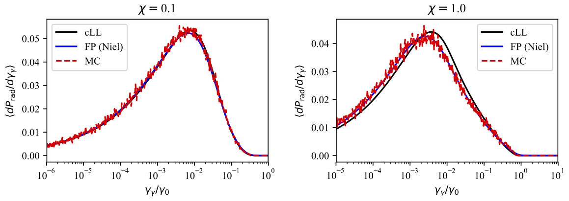
Fig. 28 Energy distribution (power spectrum) of the photon emitted by an ultra-relativistic electron bunch in a constant magnetic field. (left) for \(\chi=0.1\), (right) for \(\chi=1\).

Counter-propagating plane wave, 1D

In the benchmark benchmark/tst1d_09_rad_electron_laser_collision.py, a GeV electron bunch is initialized near the right domain boundary and propagates towards the left boundary from which a plane wave is injected. The laser has an amplitude of \(a_0 = 270\) corresponding to an intensity of \(10^{23}\ \mathrm{Wcm^{-2}}\) at \(\lambda = 1\ \mathrm{\mu m}\). The laser has a Gaussian profile of full-with at half maxium of \(20 \pi \omega_r^{-1}\) (10 laser periods). The maximal quantum parameter \(\chi\) value reached during the simulation is around 0.5.

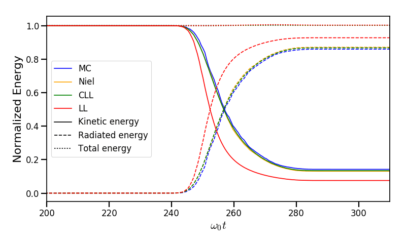
Fig. 29 Kinetic, radiated and total energy plotted respectively with solid, dashed and dotted lines for the Monte-Carlo (MC), Niel (Niel), corrected Landau-Lifshitz (CLL) and the Landau-Lifshitz (LL) models.

Fig. 29 shows that the Monte-Carlo, the Niel and the corrected Landau-Lifshitz models exhibit very similar results in term of the total radiated and kinetic energy evolution with a final radiation rate of 80% the initial kinetic energy. The relative error on the total energy is small (\(\sim 3\times10^{-3}\)). As expected, the Landau-Lifshitz model overestimates the radiated energy because the interaction happens mainly in the quantum regime.

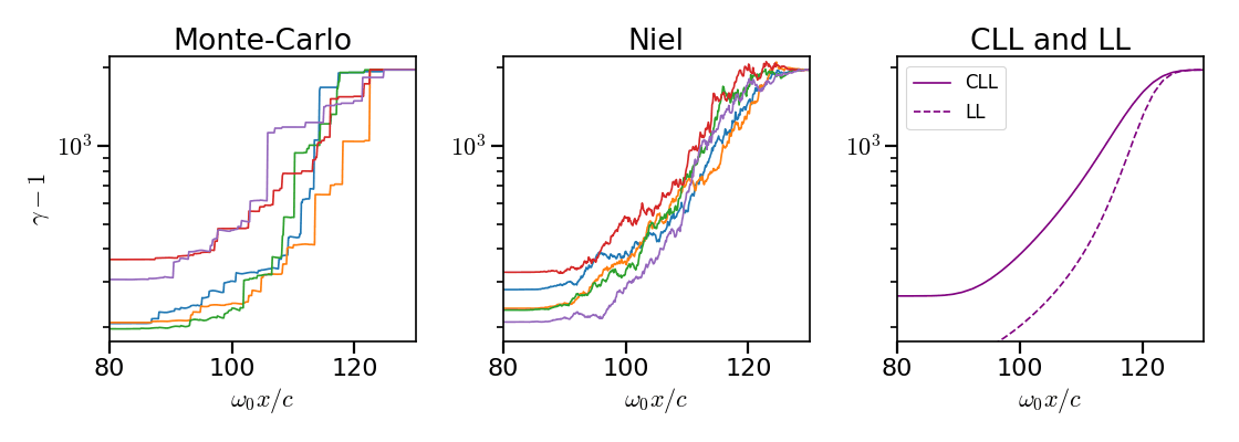
Fig. 30 Evolution of the normalized kinetic energy \(\gamma - 1\) of some selected electrons as a function of their position.

Fig. 30 shows that the Monte-Carlo and the Niel models reproduce the stochastic nature of the trajectories as opposed to the continuous approaches (corrected Landau-Lifshitz and Landau-Lifshitz). In the latter, every particles initially located at the same position will follow the same trajectories. The stochastic nature of the emission for high \(\chi\) values can have consequences in term of final spatial and energy distributions. Not shown here, the Niel stochastic model does not reproduce correctly the moment of order 3 as explained in [Niel2018a].

Synchrotron, 2D

A bunch of electrons of initial momentum \(p_{-,0}\) evolves in a constant magnetic field \(B\) orthogonal to their initial propagation direction. In such a configuration, the electron bunch is supposed to rotate endlessly with the same radius \(R = p_{-,0} /e B\) without radiation energy loss. Here, the magnetic field is so strong that the electrons radiate their energy as in a synchrotron facility. In this setup, each electron quantum parameter depends on their Lorentz factors \(\gamma_{-}\) according to \(\chi_{-} = \gamma_{-} B /m_e E_s\). The quantum parameter is maximum at the beginning of the interaction. The strongest radiation loss are therefore observed at the beginning too. As energy decreases, radiation loss becomes less and less important so that the emission regime progressively move from the quantum to the classical regime.

Similar simulation configuration can be found in the benchmarks. It corresponds to two different input files in the benchmark folder:

• tst2d_08_synchrotron_chi1.py: tests and compares the corrected Landau-Lifshitz and the Monte-Carlo model for an initial \(\chi = 1\).

• tst2d_09_synchrotron_chi0.1.py: tests and compares the corrected Landau-Lifshitz and the Niel model for an initial \(\chi = 0.1\).

In this section, we focus on the case with initial quantum parameter \(\chi = 0.1\). The magnetic field amplitude is \(B = 90 m \omega_r / e\). The initial electron Lorentz factor is \(\gamma_{-,0} = \varepsilon_{-,0}/mc^2 = 450\). Electrons are initialized with a Maxwell-Juttner distribution of temperature \(0.1 m_e c^2\).

Fig. 31 shows the time evolution of the particle kinetic energy, the radiated energy and the total energy. All radiation models provide similar evolution of these integrated quantities. The relative error on the total energy is between \(2 \times 10^{-9}\) and \(3 \times 10^{-9}\).

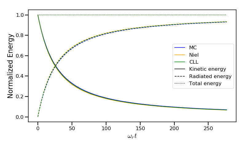
Fig. 31 Kinetic, radiated and total energies plotted respectively with solid, dashed and dotted lines for various models.

The main difference between models can be understood by studying the particle trajectories and phase spaces. For this purpose, the local kinetic energy spatial-distribution at \(25 \omega_r^{-1}\) is shown in Fig. 32 for the different models. With continuous radiation energy loss (corrected Landau-Lifshitz case), each electron of the bunch rotates with a decreasing radius but the bunch. Each electron of similar initial energies have the same trajectories. In the case of a cold bunch (null initial temperature), the bunch would have kept its original shape. The radiation with this model only acts as a cooling mechanism. In the cases of the Niel and the Monte-Carlo radiation models, stochastic effects come into play and lead the bunch to spread spatially. Each individual electron of the bunch, even with similar initial energies, have different trajectories depending on their emission history. Stochastic effects are particularly strong at the beginning with the highest \(\chi\) values when the radiation recoil is the most important.

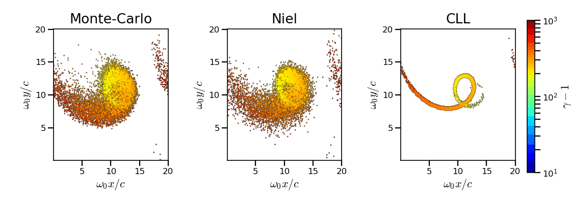
Fig. 32 Average normalized kinetic energy at time \(25 \omega_r^{-1}\) for the simulations with the Monte-Carlo, the Niel and the corrected Landau-Lifshitz (CLL) models.

Fig. 33 shows the time evolution of the electron Lorentz factor distribution (normalized energy) for different radiation models. At the beginning, the distribution is extremely broad due to the Maxwell-Juttner parameters. The average energy is well around \(\gamma_{-,0} = \varepsilon_{-,0}/mc^2 = 450\) with maximal energies above \(\gamma_{-} = 450\).

In the case of a initially-cold electron beam, stochastic effects would have lead the bunch to spread energetically with the Monte-Carlo and the Niel stochastic models at the beginning of the simulation. This effect is hidden since electron energy is already highly spread at the beginning of the interaction. This effect is the strongest when the quantum parameter is high in the quantum regime.

In the Monte-Carlo case, some electrons have lost all their energy almost immediately as shown by the lower part of the distribution below \(\gamma_{-} = 50\) after comparison with the Niel model.

Then, as the particles cool down, the interaction enters the semi-classical regime where energy jumps are smaller. In the classical regime, radiation loss acts oppositely to the quantum regime. It reduces the spread in energy and space. In the Landau-Lifshitz case, this effect starts at the beginning even in the quantum regime due to the nature of the model. For a initially-cold electron bunch, there would not have been energy spread at the beginning of the simulation. All electron would have lost their energy in a similar fashion (superimposed behavior). This model can be seen as the average behavior of the stochastic ones of electron groups having the same initial energy.

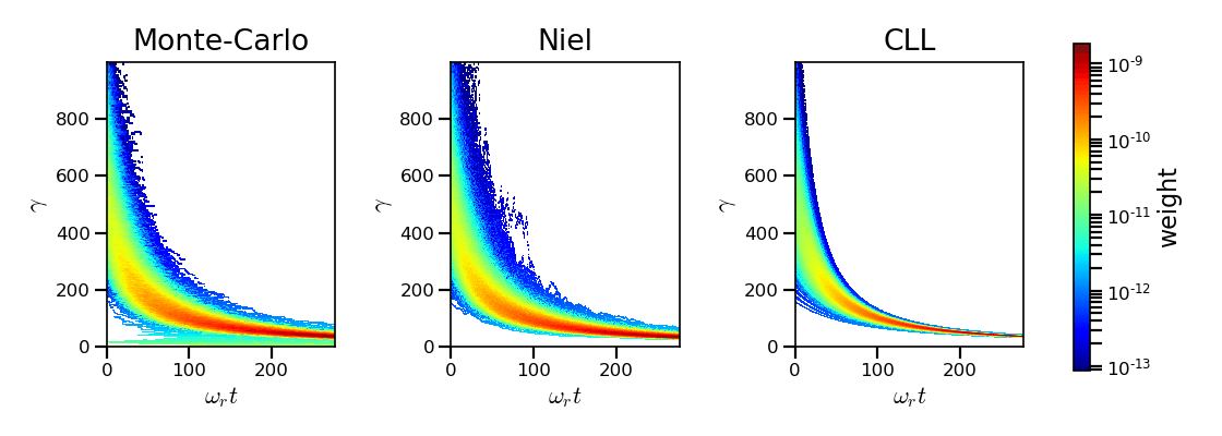
Fig. 33 Time evolution of the electron energy distribution for the Monte-Carlo, the Niel and the corrected Landau-Lifshitz (CLL) models.

Thin foil, 2D

This case is not in the list of available benchmarks but we decided to present these results here as an example of simulation study. An extremely intense plane wave in 2D interacts with a thin, fully-ionized carbon foil. The foil is located 4 µm from the left border (\(x_{min}\)). It starts with 1 µm of linear pre-plasma density, followed by 3 µm of uniform plasma of density 492 times critical. The target is irradiated by a gaussian plane wave of peak intensity \(a_0 = 270\) (corresponding to \(10^{23}\ \mathrm{Wcm^{-2}}\)) and of FWHM duration 50 fs. The domain has a discretization of 64 cells per µm in both directions x and y, with 64 particles per cell. The same simulation has been performed with the different radiation models.

Electrons can be accelerated and injected in the target along the density gradient through the combined action of the transverse electric and the magnetic fields (ponderomotive effects). In the relativistic regime and linear polarization, this leads to the injection of bunches of hot electrons every half laser period that contribute to heat the bulk. When these electrons reach the rear surface, they start to expand in the vacuum, and, being separated from the slow ion, create a longitudinal charge-separation field. This field, along the surface normal, has two main effects:

• It acts as a reflecting barrier for electrons of moderate energy (refluxing electrons).

• It accelerates ions located at the surface (target normal sheath acceleration, TNSA).

At the front side, a charge separation cavity appears between the electron layer pushed forward by the ponderomotive force and ions left-behind that causes ions to be consequently accelerated. This strong ion-acceleration mechanism is known as the radiation pressure acceleration (RPA) or laser piston.

Under the action of an extremely intense laser pulse, electrons accelerated at the target front radiate. It is confirmed in Fig. 34 showing the distribution of the quantum parameter \(\chi\) along the x axis for the Monte-Carlo, the Niel and the corrected Landau-Lifshitz (CLL) radiation models. The maximum values can be seen at the front where the electrons interact with the laser. Radiation occurs in the quantum regime \(\chi > 0.1\). Note that there is a second peak for \(\chi\) at the rear where electrons interact with the target normal sheath field. The radiation reaction can affect electron energy absorption and therefore the ion acceleration mechanisms.

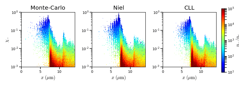
Fig. 34 \(x - \chi\) electron distribution at time 47 fs for the Monte-Carlo, the Niel and the corrected Landau-Lifshitz (CLL) model.

The time evolutions of the electron kinetic energy, the carbon ion kinetic energy, the radiated energy and the total absorbed energy are shown in Fig. 35. The corrected-Landau-Lifshitz, the Niel and the Monte-Carlo models present very similar behaviors. The absorbed electron energy is only slightly lower in the Niel model. This difference depends on the random seeds and the simulation parameters. The radiated energy represents around 14% of the total laser energy. The classical Landau-Lifshitz model overestimates the radiated energy; the energy absorbed by electrons and ions is therefore slightly lower. In all cases, radiation reaction strongly impacts the overall particle energy absorption showing a difference close to 20% with the non-radiative run.

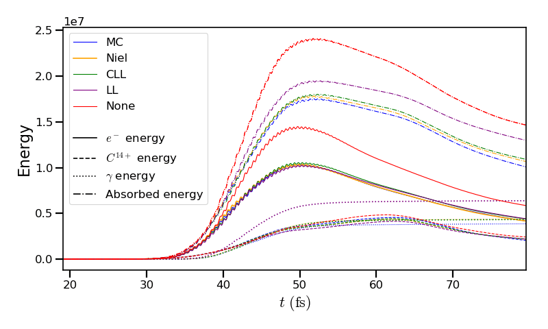
Fig. 35 Time evolution of the electron kinetic energy (solid lines), the carbon ion kinetic energy (dashed line), the radiated energy (dotted line) and the total absorbed energy by particle and radiation (dotted-dashed lines), for various models.

The differences between electron \(p_x\) distributions are shown in Fig. 36. Without radiation reaction, electrons refluxing at the target front can travel farther in vacuum (negative \(p_x\)) before being injected back to the target. With radiation reaction, these electrons are rapidly slowed down and newly accelerated by the ponderotive force. Inside the target, accelerated bunches of hot electrons correspond to the regular positive spikes in \(p_x\) (oscillation at \(\lambda /2\)). The maximum electron energy is almost twice lower with radiation reaction.

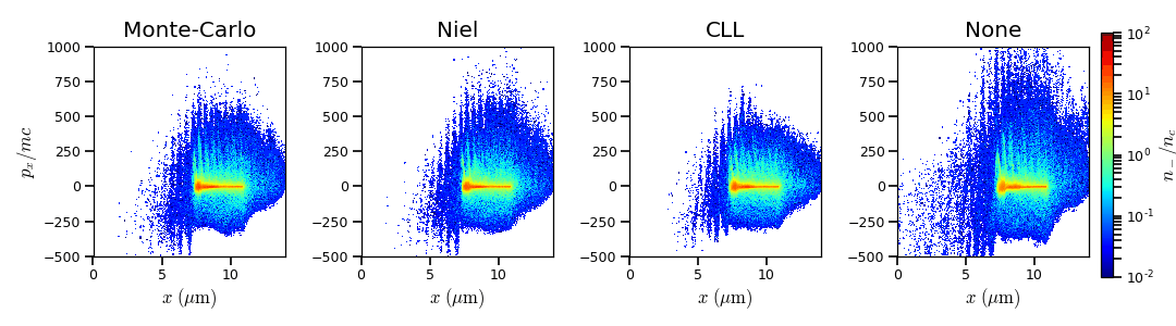
Fig. 36 \(x - p_x\) electron distribution at time 47 fs for the Monte-Carlo, the Niel, the corrected Landau-Lifshitz (CLL) model and without radiation loss (none).

---

Performances

The cost of the different models is summarized in Table 4. Reported times are for the field projection, the particle pusher and the radiation reaction together. Percentages correspond to the overhead induced by the radiation module in comparison to the standard PIC pusher.

All presented numbers are not generalizable and are only indicated to give an idea of the model costs. The creation of macro-photons is not enabled for the Monte-Carlo radiation process.

Table 4 Radiation model performances

Radiation model	None	LL	CLL	Niel	MC
Counter-propagating Plane Wave 1D Haswell (Jureca)	0.2s	0.23s	0.24s	0.26s	0.3s
Synchrotron 2D Haswell (Jureca) \(\chi=0.05\), \(B=100\)	10s	11s	12s	14s	15s
Synchrotron 2D Haswell (Jureca) \(\chi=0.5\), \(B=100\)	10s	11s	12s	14s	22s
Synchrotron 2D KNL (Frioul) \(\chi=0.5\), \(B=100\)	21s	23s	23s	73s	47s
Interaction with a carbon thin foil 2D Sandy Bridge (Poincare)	6.5s	6.5s	6.6s	6.8s	6.8s

Descriptions of the cases:

• Counter-propagating Plane Wave 1D: run on a single node of Jureca with 2 MPI ranks and 12 OpenMP threads per rank.

• Synchrotron 2D: The domain has a dimension of 496x496 cells with 16 particles per cell and 8x8 patches. A 4th order B-spline shape factor is used for the projection. The first case has been run on a single Haswell node of Jureca with 2 MPI ranks and 12 OpenMP threads per rank. the second one has been run on a single KNL node of Frioul configured in quadrant cache using 1 MPI rank and 64 OpenMP threads. On KNL, the KMP_AFFINITY is set to fine and scatter.

Only the Niel model provides better performance with a compact affinity.

• Thin foil 2D: The domain has a discretization of 64 cells per \(\mu\mathrm{m}\) in both directions, with 64 particles per cell. The case is run on 16 nodes of Poincare with 2 MPI ranks and 8 OpenMP threads per rank.

The LL and CLL models are vectorized efficiently. These radiation reaction models represent a small overhead to the particle pusher.

The Niel model implementation is split into several loops to be partially vectorized. The table lookup is the only phase that can not be vectorized. Using a fit function enables to have a fully vectorized process. The gain depends on the order of the fit. The radiation process with the Niel model is dominated by the normal distribution random draw.

The Monte-Carlo pusher is not vectorized because the Monte-Carlo loop has not predictable end and contains many if-statements. When using the Monte-Carlo radiation model, code performance is likely to be more impacted running on SIMD architecture with large vector registers such as Intel Xeon Phi processors. This can be seen in Table 4 in the synchrotron case run on KNL.

---

References

DiPiazza2012

Di Piazza et al. (2012), Rev. Mod. Phys. 84, 1177

Duclous2011(1,2)

Duclous, Kirk and Bell (2011), Plasma Physics and Controlled Fusion, 53 (1), 015009

Elkina2011

Elkina et al. (2011), Physical Review Accelerators and Beam, 14, 054401

Landau1947

Landau and Lifshitz (1947), The classical theory of fields. Butterworth-Heinemann

Lobet2013(1,2)

Lobet et al. (2016), J. Phys.: Conf. Ser. 688, 012058

Lobet2015(1,2)

Lobet (2015), Effets radiatifs et d’électrodynamique quantique dans l’interaction laser-matière ultra-relativiste (2015)

Ridgers2017

Ridgers et al. (2017), Journal of Plasma Physics, 83(5)

Ritus1985

Ritus (1985), Journal of Soviet Laser Research, 6, 497, ISSN 0270-2010

Tamburini2010

Tamburini et al. (2010), New J. Phys. 12, 123005

Timokhin2010

Timokhin (2010), Monthly Notices of the Royal Astronomical Society, 408 (4), 2092, ISSN 1365-2966