
Binary collisions & reactions
Relativistic binary collisions between particles have been implemented in Smilei following these references:
[Perez2012]: overview of the technique.
[Nanbu1997] and [Nanbu1998]: the original approach.
[Sentoku2008], [Lee1984] and [Frankel1979]: additional information.
The correction suggested in [Higginson2020] has been applied since v4.5.
[to be published] A correction for the screening of bound electrons. This makes a significant difference for weakly-ionized atoms.
This collision scheme can host reactions between the colliding macro-particles, when requested:
Ionization of an atom by collision with an electron.
Nuclear reaction between two atoms.
Please refer to that doc for an explanation of how to add collisions in the namelist file.
The binary collision scheme
Collisions are calculated at each timestep and for each collision block given in the input file:
Macro-particles that should collide are randomly paired.
Average parameters are calculated (densities, etc.).
For each pair:
Calculate the momenta in the center-of-mass (COM) frame.
Calculate the coulomb log if requested (see [Perez2012]).
If the collision corresponds to a nuclear reaction (optional), the reaction probability is computed and new particles are created if successful.
Calculate the collision rate.
Randomly pick the deflection angle.
Deflect particles in the COM frame and switch back to the laboratory frame.
If the collision corresponds to ionization (optional), its probability is computed and new electrons are created if successful.
Modifications in Smilei
A typo from [Perez2012] is corrected: in Eq. (22), corresponding to the calculation of the Coulomb Logarithm, the last parenthesis is written as a squared expression, but should not.
The deflection angle distribution given by [Nanbu1997] (which is basically a fit from Monte-Carlo simulations) is modified for better accuracy and performance. Given Nanbu’s \(s\) parameter and a random number \(U\in [0,1]\), the deflection angle \(\chi\) is:
\[\begin{split}\sin^2\frac\chi 2 = \begin{cases} \alpha U/\sqrt{1-U + \alpha^2 U} &, s < 4\\ 1-U &, \textrm{otherwise} \end{cases}\end{split}\]where \(\alpha = 0.37 s-0.005 s^2-0.0064 s^3\).
Test cases for collisions
1. Beam relaxation
An electron beam with narrow energy spread enters an ion background with \(T_i=10\) eV. The ions are of very small mass \(m_i=10 m_e\) to speed-up the calculation. Only e-i collisions are calculated. The beam gets strong isotropization => the average velocity relaxes to zero.
Three figures show the time-evolution of the longitudinal \(\left<v_\|\right>\) and transverse velocity \(\sqrt{\left<v_\perp^2\right>}\)
Fig. 14 : initial velocity = 0.05, ion charge = 1
Fig. 15 : initial velocity = 0.01, ion charge = 1
Fig. 16 : initial velocity = 0.01, ion charge = 3
Each of these figures show 3 different blue and red curves which correspond to different ratios of particle weights: 0.1, 1, and 10.
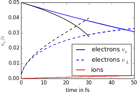
Fig. 14 Relaxation of an electron beam. Initial velocity = 0.05, ion charge = 1.
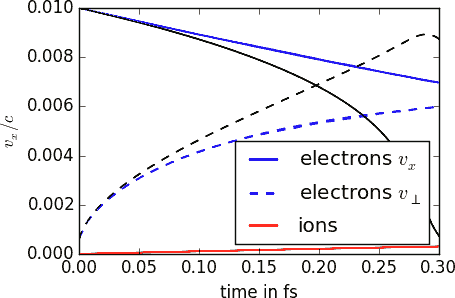
Fig. 15 Relaxation of an electron beam. Initial velocity = 0.01, ion charge = 1.
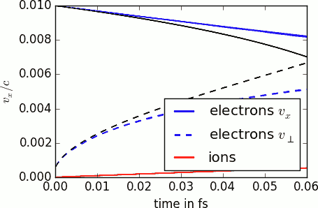
Fig. 16 Relaxation of an electron beam. Initial velocity = 0.01, ion charge = 3.
The black lines correspond to the theoretical rates taken from the NRL formulary:
The distribution is quickly non-Maxwellian so that theory is valid only at the beginning.
2. Thermalization
A population of electrons has a different temperature from that of the ion population. Through e-i collisions, the two temperatures become equal. The ions are of very small mass \(m_i=10 m_e\) to speed-up the calculation. Three cases are simulated, corresponding to different ratios of weights: 0.2, 1 and 5. They are plotted in Fig. 17.
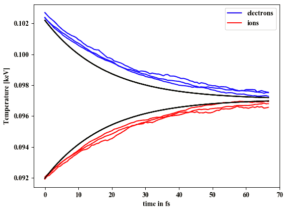
Fig. 17 Thermalization between two species.
The black lines correspond to the theoretical rates taken from the NRL formulary:
3. Temperature isotropization
Electrons have a longitudinal temperature different from their transverse temperature. They collide only with themselves (intra-collisions) and the anisotropy disappears as shown in Fig. 18.
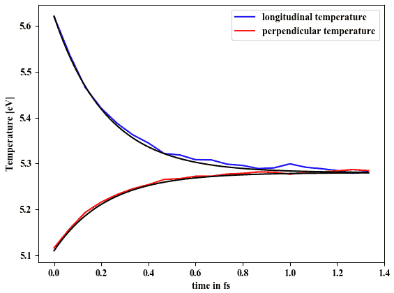
Fig. 18 Temperature isotropization of an electron population.
The black lines correspond to the theoretical rates taken from the NRL formulary:
4. Maxwellianization
Electrons start with zero temperature along \(y\) and \(z\). Their velocity distribution along \(x\) is rectangular. They collide only with themselves and the rectangle becomes a maxwellian as shown in Fig. 19.
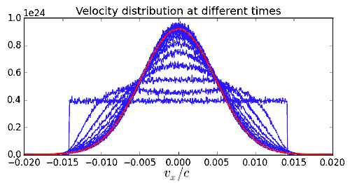
Fig. 19 Maxwellianization of an electron population. Each blue curve is the distribution at a given time. The red curve is an example of a gaussian function.
5. Stopping power
Test electrons (very low density) collide with background electrons of density \(10\,n_c\) and \(T_e=5\) keV. Depending on their initial velocity, they are slowed down at different rates, as shown in Fig. 20.
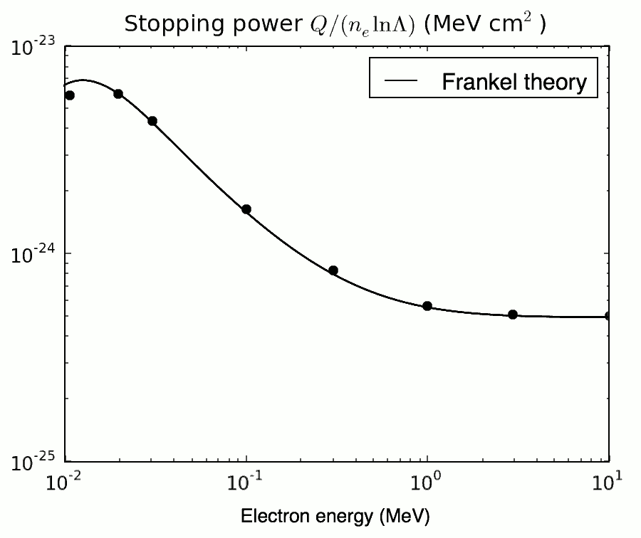
Fig. 20 Stopping power of test electrons into a background electron population. Each point is one simulation. The black line is Frankel’s theory [Frankel1979].
6. Conductivity
Solid-density Cu is simulated at different temperatures (e-i equilibrium) with only e-i collisions. An electric field of \(E=3.2\) GV/m (0.001 in code units) is applied using two charged layers on each side of the solid Cu. The electron velocity increases until a limit value \(v_f\). The resulting conductivity \(\sigma=en_ev_f/E\) is compared in Fig. 21 to the models in [Lee1984] and [Perez2012].
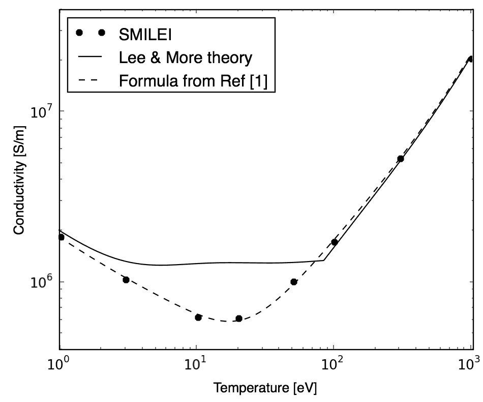
Fig. 21 Conductivity of solid-density copper. Each point is one simulation.
Collisional ionization
The binary collisions can also be ionizing if they are electron-ion collisions. The approach is almost the same as that provided in [Perez2012].
When ionization is requested by setting ionizing=True, a few additional operations
are executed:
At the beginning of the run, cross-sections are calculated from tabulated binding energies (available for ions up to atomic number 100). These cross-sections are then tabulated for each requested ion species.
Each timestep, the particle density \(n = n_e n_i/n_{ei}\) (similar to the densities above for collisions) is calculated.
During each collision, a probability for ionization is computed. If successful, the ion charge is increased, the incident electron is slowed down, and a new electron is created.
Warnings
This scheme does not account for recombination, which would balance ionization over long time scales.
Relativistic change of frame
A modification has been added to the theory of [Perez2012] in order to account for the laboratory frame being different from the ion frame. Considering \(\overrightarrow{p_e}\) and \(\overrightarrow{p_i}\) the electron and ion momenta in the laboratory frame, and their associated Lorentz factors \(\gamma_e\) and \(\gamma_i\), we define \(\overrightarrow{q_e}=\overrightarrow{p_e}/(m_e c)\) and \(\overrightarrow{q_i}=\overrightarrow{p_i}/(m_i c)\). The Lorentz factor of the electron in the ion frame is \(\gamma_e^\star=\gamma_e\gamma_i-\overrightarrow{q_e}\cdot\overrightarrow{q_i}\). The probability for ionization reads:
where \(v_e\) is the electron velocity in the laboratory frame, \(\sigma\) is the cross-section in the laboratory frame, \(\sigma^\star\) is the cross-section in the ion frame, and \(V^\star=c\sqrt{\gamma_e^{\star\,2}-1}/(\gamma_e\gamma_i)\).
The loss of energy \(m_ec^2 \delta\gamma\) of the incident electron translates into a change in momentum \({q_e^\star}' = \alpha_e q_e^\star\) in the ion frame, with \(\alpha_e=\sqrt{(\gamma_e^\star-\delta\gamma)^2-1}/\sqrt{\gamma_e^{\star2}-1}\). In the laboratory frame, it becomes \(\overrightarrow{q_e'}=\alpha_e\overrightarrow{q_e}+((1-\alpha_e)\gamma_e^\star-\delta\gamma)\overrightarrow{q_i}\).
A similar operation is done for defining the momentum of the new electron in the lab frame. It is created with energy \(m_ec^2 (\gamma_w-1)\) and its momentum is \(q_w^\star = \alpha_w q_e^\star\) in the ion frame, with \(\alpha_w=\sqrt{\gamma_w^2-1}/\sqrt{\gamma_e^{\star 2}-1}\). In the laboratory frame, it becomes \(\overrightarrow{q_w}=\alpha_w\overrightarrow{q_e}+(\gamma_w-\alpha_w\gamma_e^\star)\overrightarrow{q_i}\).
Multiple ionization
A modification has been added to the theory of [Perez2012] in order to account for multiple ionization in a single timestep. The approach for field ionization by Nuter et al has been adapted to calculate the successive impact ionization probabilities when an ion is ionized several times in a row.
Writing the probability to not ionize an ion already ionized \(i\) times as \(\bar{P}^i = \exp\left( -W_i\Delta t\right)\), and defining \(R^m_n = (1-W_m/W_n)^{-1}\), we can calculate the probability to ionize \(k\) times the ion:
To simplify the calculation of \(P^i_k\) (in particular the second case in the equation above) we use the following equivalent expression:
where \(A_k = \prod\limits_{j=0}^{k} W_{i+j}\) and \(B_k^p = \prod\limits_{j=0,j\ne p}^{k} (W_{i+j}-W_{i+p})\). These two quantities can be computed recursively for each \(k\).
The cumulative probability \(F^i_k = \sum_{j=0}^{k} P^i_j\) provides an efficient way to pick when the ionization stops: we pick a random number \(U\in [0,1]\) and loop from \(k=0\) to \(k_\mathrm{max}\). We stop ionizing when \(F^i_k>U\).
Test cases for ionization
1. Ionization rate
A cold plasma of \(\mathrm{Al}^{3+}\) is set with density \(n_e=10^{21} \mathrm{cm}^{-3}\) and with all electrons drifting at a velocity \(v_e=0.03\,c\). The charge state of ions versus time is shown in Fig. 22 where the three dotted curves correspond to three different weight ratios between electrons and ions.
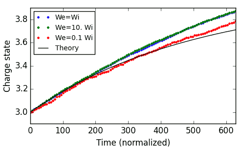
Fig. 22 Ionization of an aluminium plasma by drifting electrons.
The theoretical curve (in black) corresponds to \(1-\exp\left(v_en_e\sigma t\right)\) where \(\sigma\) is the ionization cross section of \(\mathrm{Al}^{3+}\) at the right electron energy. The discrepancy at late time is due to the changing velocity distributions and to the next level starting to ionize.
2. Inelastic stopping power
A cold, non-ionized Al plasma is set with density \(n_e=10^{21} \mathrm{cm}^{-3}\). Electrons of various initial velocities are slowed down by ionizing collisions and their energy loss is recorded as a function of time.
A few examples are given in the left graph of Fig. 23. The theoretical curve is obtained from [Rohrlich1954]. Note that this theory does not work below a certain average ionization energy, in our case \(\sim 200\) eV.
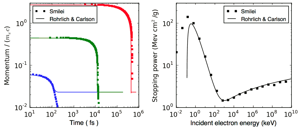
Fig. 23 Left: ionization slowing down versus time, for electrons injected at various initial energies into cold Al. Right: corresponding stopping power versus initial electron energy.
In the same figure, the graph on the right-hand-side provides the stopping power value in the same context, at different electron energies. It is compared to the same theory.
3. Multiple ionization
If the timestep is large, multiple ionization can occur, especially with cold high-Z material and high-energy electrons. The multiple ionization algorithm is not perfect, as it does not shuffle the particles for each ionization. Thus, good statistical sampling is reached after several timesteps. To test the potential error, we ran simulations of electrons at 1 MeV incident on cold atoms. The evolution of the secondary electron density is monitored versus time in Fig. 24.
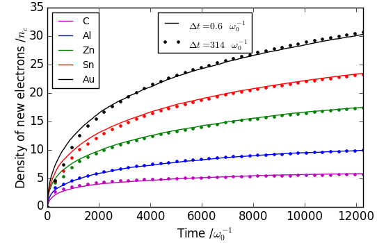
Fig. 24 Secondary electron density vs time, for cold plasmas traversed by a 1 MeV electron beam.
The solid lines correspond to a very-well resolved ionization, whereas the dashed lines correspond to a large timestep. A difference is visible initially, but decreases quickly as the statistical sampling increases and as the subsequent ionization cross-sections decrease.
3. Effect of neglecting recombination
As recombination is not accounted for, we can expect excess ionization to occur indefinitely without being balanced to equilibrium. However, in many cases, the recombination rate is small and can be neglected over the duration of the simulation. We provide an example that is relevant to picosecond-scale laser-plasma interaction. Plasmas initially at a density of 10 times the critical density are given various initial temperatures. Ionization initially increases while the temperature decreases, until, after a while, their charge state stagnates (it still increases, but very slowly). In Fig. 25, these results are compared to a Thomas-Fermi model from [Desjarlais2001].
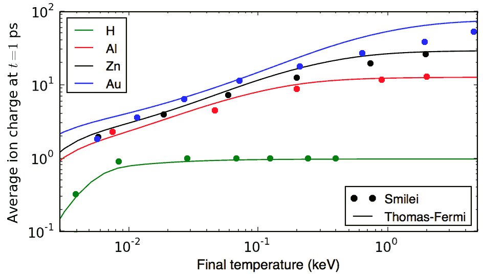
Fig. 25 Final charge state of various plasmas at various temperatures.
The model does not account for detailed ionization potentials. It provides a rough approximation, and is particularly questionable for low temperatures or high Z. We observe that Smilei’s approach for impact ionization provides decent estimates of the ionization state. Detailed comparison to atomic codes has not been done yet.
Bound electron screening
The Coulomb potential that is assumed in the collision theory of Nanbu does not correctly apply to neutral atoms or weakly-ionized ions. Indeed, in addition to the screening caused by free electrons (Debye screening), the potential must account for the bound-electron screening.
In Smilei, a simple model is available in the case of electron-ion collisions. It relies on the Thomas-Fermi characteristic length \(\lambda_{TF} = (9\pi^2/16Z)^{1/3}a_0\), where \(a_0\) is the Bohr radius, to describe the extent of the screening aroud the nucleus. With a few approximations, the model suggests to replace, in the collisional frequency, the term \(Z^{\star 2}\ln\Lambda_D\) by
where \(\ln\Lambda_D\) is the usual (Debye-screening) Coulomb logarithm, and \(\Lambda_{TF} = \lambda_{TF}\Lambda_D /\lambda_D\). This approach is basic but captures the essential trend. Little data for comparison is available for weakly-ionized atoms, but the collision cross-sections are well-known for neutral atoms. Fig. 26 shows a comparison between the model implemented in Smilei and the theoretical cross-sections calculated by the code ELSEPA [Salvat2005].
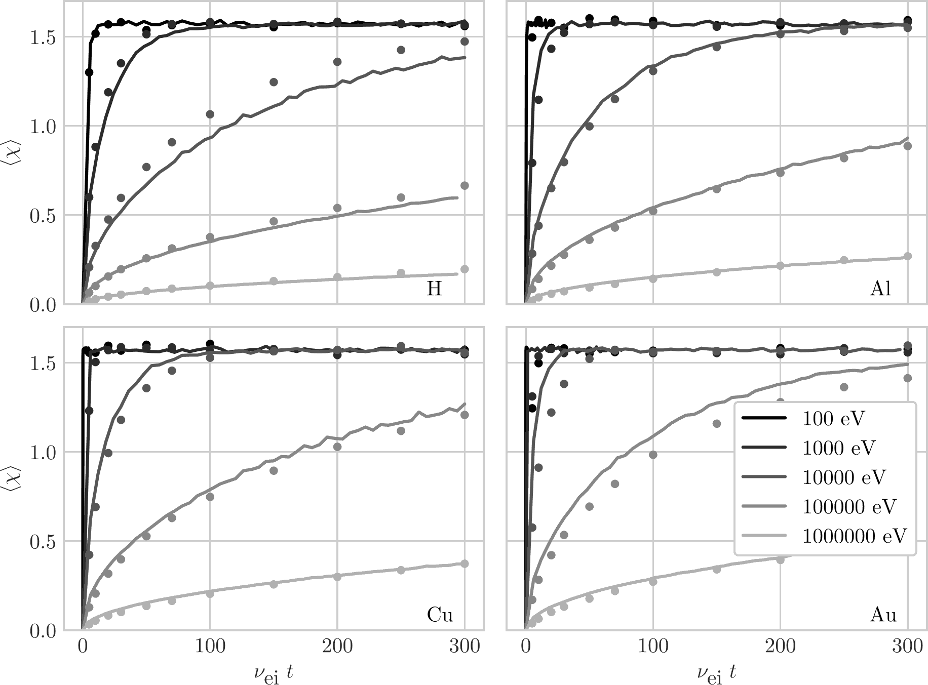
Fig. 26 Average deflection angle vs. time for collisions between electrons and neutral atoms. The lines correspond to Smilei simulations with various electron beam energy, and the dots are calculated from the theoretical code ELSEPA.
Nuclear reactions
Nuclear reactions may occur during collisions when requested. The reaction scheme is largely inspired from [Higginson2019].
1. Outline of the nuclear reaction process
We take advantage of the relativistic kinematics calculations of the binary collision scheme to introduce the nuclear reactions in the COM frame:
The cross-section \(\sigma\) (tabulated for some reactions) is interpolated, given the kinetic energies.
The probability for the reaction to occur is calculated.
This probability is randomly sampled and, if successful:
New macro-particles (the reaction products) are created.
Their angle is sampled from a tabulated distribution.
Their mpmenta are calculated from the conservation of total energy and momentum.
Their momenta are boosted back to the simulation frame.
Otherwise: the collision process proceeds as usual.
2. Nuclear reaction probability
The probability for the reaction to occur is calculated as \(P=1-\exp(R\, v\, n\, \sigma\, \Delta t)\) where v is the relative velocity, n is a corrected density (see [Higginson2020]), and R is a rate multiplier (see [Higginson2019]).
This factor R is of great importance for most applications, because almost no reactions would occur when \(R=1\). This factor artificially increases the number of reactions to ensure enough statistics. The weights of the products are adjusted accordingly, and the reactants are not destroyed in the process: we simply decrease their weight by the same amount.
In Smilei, this factor R can be forced by the user to some value, but by default, it is automatically adjusted so that the final number of created particles approches the initial number of pairs.
3. Creation of the reaction products
Special care must be taken when creating new charged particles while conserving Poisson’s equation. Following Ref. [Higginson2019], we choose to create two macro-particles of each type. To explain in detail, let us write the following reaction:
Two particles of species 3 are created: one at the position of particle 1, the other at the position of particle 2. Two particles of species 4 are also created. To conserve the charge at each position, the weights of the new particles must be:
where \(w\) is the products’ weight, and the \(q_i\) are the charges.
4. Calculation of the resulting momenta
The conservation of energy reads:
where the \(K_i\) are kinetic energies, and \(Q\) is the reaction’s Q-value. In the COM frame, we have, by definition, equal momenta: \(p_3 = p_4\). Using the relativistic expression \((K_k+m_k)^2=p_k^2+m_k^2\), we can calculate that
Substituting for \(K_4\) using the conservation of energy, this translates into
where we have defined \(A_{ij}=K_1 + K_2 +Q+i\,m_3+j\,m_4\). We thus obtain
Finally,
which expresses the resulting momentum as a function of the initial energies.
Collisions debugging
Using the parameter debug_every in a Collisions() group (see Collisions & reactions)
will create a file with info about these collisions.
These information are stored in the files “Collisions0.h5”, “Collisions1.h5”, etc.
- The hdf5 files are structured as follows:
One HDF5 file contains several groups called
"t********"where"********"is the timestep. Each of these groups contains several arrays, which represent quantities vs. space.
The available arrays are:
s: defined in [Perez2012]: \(s=N\left<\theta^2\right>\), where \(N\) is the typical number of real collisions during a timestep, and \(\left<\theta^2\right>\) is the average square deviation of individual real collisions. This quantity somewhat represents the typical amount of angular deflection accumulated during one timestep. It is recommended that \(s<1\) in order to have realistic collisions.
coulomb_log: average Coulomb logarithm.
debyelength: Debye length (not provided if all Coulomb logs are manually defined).
The arrays have the same dimension as the plasma, but each element of these arrays is an average over all the collisions occurring in a single patch.