Multiphoton Breit-Wheeler pair creation

The multiphoton Breit-Wheeler (\(\gamma + n\omega \rightarrow e^- + e^+\)), also referred to as the nonlinear Breit-Wheeler, corresponds to the decay of a high-energy photon into a pair of electron-positron when interacting with a strong electromagnetic field.

In the vacuum, the electromagnetic field becomes nonlinear from the Schwinger electric field \(E_s = 1.3 \times 10^{18}\ \mathrm{V/m}\) corresponding to an intensity of \(10^{29}\ \mathrm{Wcm^{-2}}\) for \(\lambda = 1\ \mu m\). In such a field, spontaneous apparitions of electron-positron pairs from the nonlinear vacuum are possible. If this field is not reachable in the laboratory frame, it will be very close in the boosted frame of highly-accelerated electrons. At \(10^{24}\ \mathrm{Wcm^{-2}}\), a Lorentz factor of \(\gamma \sim 10^5\) is required to reach the Schwinger limit. This is the reason why quantum electrodynamics effects and in particular strong- field pair generation is accessible with the extreme-intensity lasers (multipetawatt lasers).

As for electrons or positrons, the strength of QED effects depends on the photon quantum parameter:

(35)\[\chi_\gamma = \frac{\gamma_\gamma}{E_s} \sqrt{ \left( \mathbf{E}_\perp + \mathbf{c} \times \mathbf{B} \right)^2 }\]

where \(\gamma_\gamma = \varepsilon_\gamma / m_e c^2\) is the photon normalized energy, \(m_e\) the electron mass, \(c\) the speed of light in vacuum, \(\mathbf{E}_\perp\) is the electric field orthogonal to the propagation direction of the photon, \(\mathbf{B}\) the magnetic field.

---

Physical model

The energy distribution of the production rate of pairs by a hard photon is given by the Ritus formulae

(36)\[\frac{d^2N_{BW}}{d \chi_{\pm} dt} = \frac{\alpha_f m_e^2 c^4}{\pi \sqrt{3} \hbar \varepsilon_\gamma \chi_\gamma} \int_{x}^{+\infty}{\sqrt{s} K_{1/3} \left( \frac{2}{3} s^{3/2} \right) ds - \left( 2 - \chi_\gamma x^{3/2} \right) K_{2/3} \left( \frac{2}{3} x^{3/2} \right) }\]

where \(x = \left( \chi_\gamma / (\chi_{-} \chi_{+}) \right)^{2/3}\). The parameters \(\chi_{-}\) and \(\chi_{+}\) are the respective Lorentz invariant of the electron and the positron after pair creation. Furthermore, one has \(\chi_- = \chi_\gamma - \chi_+\) meaning that \(\chi_-\) and \(\chi_+\) can be interchanged.

The total production rate of pairs can be written

(37)\[\frac{dN_{BW}}{dt} = \frac{\alpha_f m_e^2 c^4}{ \hbar \varepsilon_\gamma} \chi_\gamma T \left( \chi_\gamma \right)\]

where

(38)\[T \left( \chi_\gamma \right) = \frac{1}{\pi \sqrt{3} \chi_\gamma^2 } \int_{0}^{+\infty}{\int_{x}^{+\infty}{\sqrt{s} K_{1/3} \left( \frac{2}{3} s^{3/2} \right) ds - \left( 2 - \chi_\gamma x^{3/2} \right) K_{2/3} \left( \frac{2}{3} x^{3/2} \right) }} d\chi_-\]

A photon of energy \(\varepsilon_\gamma\) traveling in a constant electric field \(E\) has a Lorentz parameter equal to \(\chi_\gamma = \varepsilon_\gamma E / (E_s m_e c^2)\).

We consider the case where photon interact in a constant uniform electric field. For a field of amplitude \(E = 500 m_e \omega c / e\), the energy distribution and the production rate of pair creation as a function of \(\chi_\gamma\) are plotted in Fig. 37. It shows that the total production rate of electron-positron pairs rises rapidly to reach a peak around \(\chi_\gamma = 10\) with almost a pair generated per femtosecond. Under \(\chi_\gamma = 0.1\), the production rate is very weak with less than a pair after 100 picoseconds of interaction. Above \(\chi_\gamma = 10\), the production decreases slowly with \(\chi_\gamma\).

The right subplot in Fig. 37 gives the probability for a photon to decay into a pair as a function of the energy given to the electron (using approximation \(\chi_\gamma / \chi_- = \gamma_\gamma / \gamma_-\)) for a field of amplitude \(E = 500 m_e \omega c / e\). It can also be seen as the pair creation energy distribution. The distribution is symmetric with respect to \(\chi_- / \chi_\gamma = 1/2\). Below \(\chi_\gamma = 10\), The maximum probability corresponds to equal electron-positron energies \(\chi_- = \chi_+ = \chi_\gamma / 2\). Above this threshold, the energy dispersion increases with \(\chi_\gamma\).

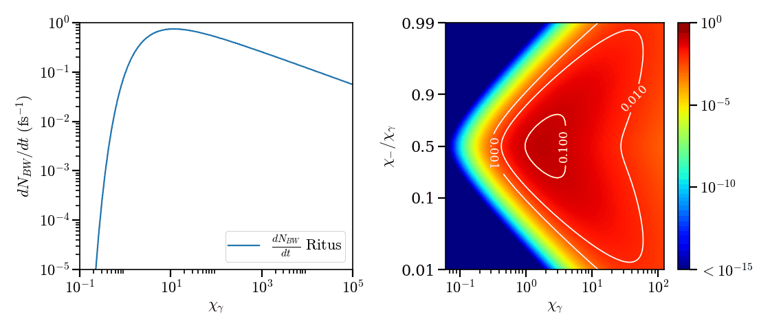
Fig. 37 (left) - Normalized total pair production distribution given by Eq. (37). (right) - Normalized pair creation \(\chi\) distribution given by Eq. (36).

---

Stochastic scheme

The Multiphoton Breit-Wheeler is treated with a Monte-Carlo process similar to the nonlinear inverse Compton Scattering (see the radiation reaction page). It is close to what has been done in [Duclous2011], [Lobet2013], [Lobet2015].

The first preliminary step consists on introducing the notion of macro-photon. Macro-photons are simply the equivalent of macro-particles (see the macro-particle section) extended to photons. There are defined by a charge and a mass equal to 0. The momentum is substituted by the photon momentum \(\mathbf{p}_\gamma = \hbar \mathbf{k}\) where \(\mathbf{k}\) is the wave vector. The momentum contains the photon energy so that \(\mathbf{p}_\gamma = \gamma_\gamma m_e \mathbf{c}\). The definition of the photon Lorentz factor is therefore also slightly different than particles.

1. An incremental optical depth \(\tau\), initially set to 0, is assigned to the macro-photon. Decay into pairs occurs when it reaches the final optical depth \(\tau_f\) sampled from \(\tau_f = -\log{(\xi)}\) where \(\xi\) is a random number in \(\left]0,1\right]\).

2. The optical depth \(\tau\) evolves according to the photon quantum parameter following:

(39)\[\frac{d\tau}{dt} = \frac{dN_{BW}}{dt}\left( \chi_\gamma \right)\]

that is also the production rate of pairs (integration of Eq. (36)).

3. The emitted electron’s quantum parameter \(\chi_-\) is computed by inverting the cumulative distribution function:

(40)\[P(\chi_-,\chi_\gamma) = \frac{\displaystyle{\int_0^{\chi_-}{ \frac{d^2N_{BW}}{d \chi dt} d\chi}}}{\displaystyle{\int_0^{\chi_\gamma}{\frac{d^2N_{BW}}{d \chi dt} d\chi}}}\]

The inversion of \(P(\chi_-,\chi_\gamma)=\xi'\) is done after drawing a second random number \(\xi' \in \left[ 0,1\right]\) to find \(\chi_-\). The positron quantum parameter is \(\chi_+ = \chi_\gamma - \chi_-\).

4. The energy of the emitted electron is then computed: \(\varepsilon_- = mc^2 \gamma_- = mc^2 \left[ 1 + \left(\gamma_\gamma - 2\right) \chi_- / \chi_\gamma \right]\). If \(\gamma_\gamma < 2\), the pair creation is not possible since the photon energy is below the rest mass of the particles.

5. The photon momentum is then updated. Propagation direction is the same as for the photon. Pairs are created at the same position as for the photon. The weight is conserved. It is possible to create more than a macro-electron or a macro-positron in order to improve the phenomenon statistics. In this case, the weight of each macro-particle is the photon weight divided by the number of emissions.

---

Implementation

C++ classes for the multiphoton Breit-Wheeler process are located in the directory src/MultiphotonBreitWheeler. In Smilei, the multiphoton Breit-Wheeler process is not incorporated in the photon pusher in order to preserve vector performance of the latter one.

Description of the files:

• Class MultiphotonBreitWheelerTables: This class initializes and manages the multiphoton Breit-Wheeler parameters. It contains the methods to read the tables and data structures to store them. It also contains default embebded tables. Then, it provides several methods to look for values in the tables for the Monte-Carlo process and compute different parameters used by this physical mechanism.

• Class MultiphotonBreitWheeler: this class contains the methods to perform the Breit-Wheeler Monte-Carlo process described in the previous section).

• Class MultiphotonBreitWheelerFactory: this class is supposed to manage the different Breit-Wheeler algorithms. For the moment, only one model is implemented.

If the multiphoton Breit-Wheeler is activated for a photon species, the factory will initialize the instance Multiphoton_Breit_Wheeler_process of the class MultiphotonBreitWheeler declared in the corresponding species (see species.cpp).

The multiphoton Breit-Wheeler Monte-Carlo process is performed in the method dynamics of species. It is called after the particle field interpolation (field gathering), after ionization and radiation reaction and before the particle pusher. At this stage, the new particles are stored in a temporary buffer called new_pair. This is an array of two instances of Particles. It is declared in Multiphoton_Breit_Wheeler_process. Particles are imported in the main species particle arrays (particles object in species) only after the current deposition and before the boundary conditions using the method importParticles of the class Particles.

---

Tables

External tables can be generated using an external tools called smilei_tables. More information can be found in Generation of the external tables.

---

Benchmarks

Synchrotron, 2D

In this configuration, a mono-energetic bunch of photons is initialized in a constant uniform strong magnetic field. The photons decay into pairs via the multiphoton Breit-Wheeler progressively. In this particular case, the generated electrons and positrons do not radiate in order to capture the emission energy spectrum. Two cases are simulated with different initial quantum parameters:

• Case 1: \(\chi_{\gamma,0} = 1\), \(B = 270\), \(\gamma_{\gamma,0} = 1500\)

• Case 2: \(\chi_{\gamma,0} = 20\), \(B = 1000\), \(\gamma_{\gamma,0} = 8125\)

The results of the first case are shown in Fig. 38. The two first figures represent respectively the electron (left) and the positron energy (center) spectrum at the end of the simulation when all photons have been converted into pairs. The last one on the right is the time evolution of the photon (green), electron (blue), positron (orange) and total (black) kinetic energy. The quantum parameter of all photons is initially equal to \(\chi_{\gamma,0} = 1\). According to Fig. 37, we are located in an area of the energy distribution where electrons and positrons are more likely to be created with almost the same energy (\(\chi_{+} = \chi_{-} =\chi_{\gamma,0} /2\)). This is confirmed in Fig. 38. Electron and positron energy spectra are well similar, symmetric and centered at half the initial photon energy equal to \(\gamma = 750\). The energy balance (right figure) shows that positron and electron kinetic energies have the same behaviors and converge to half the initial photon energy at the end of the simulation. The total energy is well constant and conserved in time.

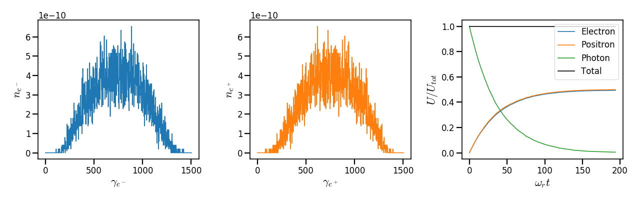
Fig. 38 (left) - Electron energy spectrum at the end of the run. (middle) - Positron energy spectrum at the end of the run. (right) - Time evolution of the photon (green), electron (blue), positron (orange) and total (black) normalized energy \(U / U_{tot}\).

The results of the second case are shown in Fig. 39 as for the first case. Here, the quantum parameter of all photons is initially equal to \(\chi_{\gamma,0} = 20\). This means that contrary to the previous case, the probability to generate electrons and positrons of similar energy is not the most significant. As in Fig. 37, the energy spectra exhibit two maximums. This maximums are located approximately at 10% and 90% of the initial photon energy of \(\gamma_{\gamma,0} = 8125\). Electron and positron spectra are nonetheless similar and symmetric in respect to half the initial photon energy. Again, the energy balance (right figure) shows that positron and electron kinetic energies have the same behaviors and converge to half the initial photon energy at the end of the simulation. The total energy is well constant and conserved in time.

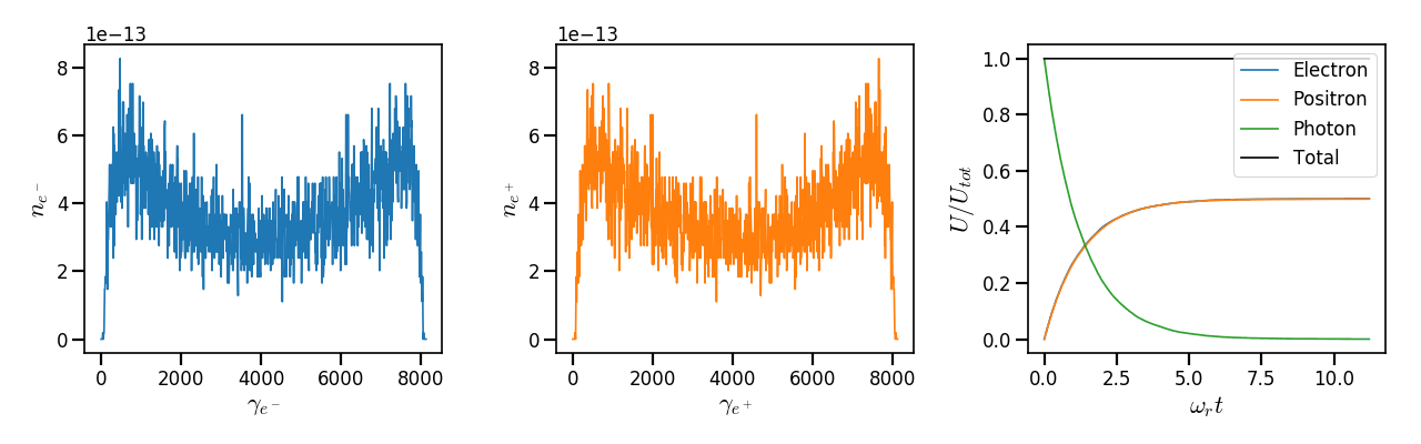
Fig. 39 (left) - Electron energy spectrum at the end of the run. (middle) - Positron energy spectrum at the end of the run. (right) - Time evolution of the photon (green), electron (blue) and positron (orange) normalized energy \(U / U_{tot}\).

The benchmark tst2d_10_multiphoton_Breit_Wheeler is very close to the second case presented here.

Counter-propagating plane wave, 1D

In this test case, a bunch of electrons is initialized at the right side of the domain with an initial energy of 4 GeV. The bunch is made to collide head-on with a laser plane wave injected from the left side of the domain. The laser has a maximal intensity of \(10^{23}\ \mathrm{Wcm^{-2}}\). It is circularly polarized and has a temporal Gaussian profile with a FWHM (full width at half maximum) of 10 periods (approximately corresponding to 33 fs). A wavelength of \(1\ \mathrm{\mu m}\) is considered.

This configuration is one of the most efficient to trigger QED effects since it maximizes the particle and photon quantum parameters.

By interacting with the laser pulse, the high-energy electron will first radiate high-energy gamma photons that will be generated as macro-photons by the code via the nonlinear Compton scattering. These photons are generated in the same direction of the electrons with an energy up to almost the electron kinetic energy. Then, the macro-photons interact in turn with the laser field and can decay into electron-positron pairs via the multiphoton Breit-Wheeler process.

The first plot on left of Fig. 40 shows the energy balance of the simulation. The second plot on the center of Fig. 40 shows the time evolution of the number of macro-electrons, macro-positrons and macro-photons. The electron bunch energy rapidly drops after entering the laser field around \(t = 240 \omega_r^{-1}\). At the same time, many macro-photons are generated by the particle number evolution as shown in Fig. 40. The photon energy therefore rapidly rises as the electron energy decreases.

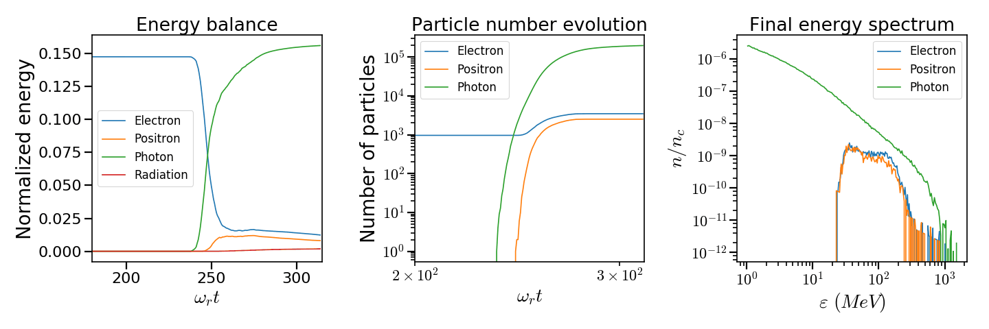
Fig. 40 (left) - Energy balance of the simulation. In the legend, Photon represents the macro-photon energy and Radiation represents the radiated energy excluding the macro-photons. (center) - Time evolution of the number of macro-electrons (blue), macro-positrons (orange) and macro-photons (green) in the simulation. (right) - Final energy spectrum of the electrons (blue), positrons (orange), and photons (green).

The multiphoton Breit-Wheeler generation of electron-positron starts latter when emitted macro-photons enters the high-intensity region of the laser. This is revealed by the yield of macro-positron. When electrons and positrons have lost sufficient energy, they can not produce macro-photons anymore and radiated energy is therefore added directly in the energy balance. This is shown by the red curve of the energy balance of Fig. 40. The radiated energy rises after the main phase of the macro-photon generation after \(t = 250 \omega_r^{-1}\). The radiated energy contains the energy from the continuous radiation reaction model and from the discontinuous Monte-Carlo if the energy of the emitted photon is below \(\gamma = 2\). Under this threshold, the photon can not decay into electron-positron pair. It is therefore useless and costly to generated a macro-photon.

The final electron, positron and photon energy spectra are shown in the right plot of Fig. 40. At the end of the simulation, the photon spectrum is a broad decreasing profile ranging from 1 MeV to 1 GeV. This is the consequence of two main facts:

• The highest is the photon energy, more important is the probability to decay into pairs.

• As electron and positron lose energy, they continue to radiate smaller ans smaller photon energy.

Electron and positron spectra are very similar ranging from 20 MeV to mainly 200 MeV. Few particles have an energy above this threshold up to 1 GeV.

This corresponds to the benchmark benchmark/tst1d_10_pair_electron_laser_collision.py.