Export to VTK and 3D visualization¶

The goal of this tutorial is to learn how to export some diagnostics to the VTK format and how to visualize them in 3D. Two simulations will be run, one in "3Dcartesian" geometry and the other in "AMcylindrical" geometry. In this tutorial we will use the open-source application Paraview to open the VTK files and 3D visualization, although this is not the only possible choice.

This tutorial is meant as a first introduction to the 3D visualization of Smilei results. For the sake of clarity, only a few available representation options will be explored, with no pretense of completeness in the field of 3D visualization or in the use of Paraview or similar software.

In particular this tutorial will explain how to

export Fields results to VTK

export the macro-particles’ coordinates in the TrackParticles results to VTK

visualize a Volume Rendering of Fields with Paraview

visualize the tracked macro-particles as points with Paraview

perform the same operations for a simulation in "AMcylindrical" geometry.

The simulations used for this tutorial is relatively heavy so make sure to submit the job on 40 cores at least to run in a few minutes. This tutorial needs an installation of the vtk Python library to export the data with happi. The export in 3D of data obtained in "AMcylindrical" geometry also requires the installation of the scipy Python library.

Disclaimer This tutorial is not physically relevant. Proper simulations of this kind must be done with better resolution in all directions, just to start. This would give more accurate results, but it would make the simulations even more demanding.

Warning To avoid wasting computing resources it is highly recommended to start small when learning how to visualize results in 3D. Apart from the simulation generating the physically accurate data, the export and visualization of large amounts of data requires resources and computing time. For these reasons, if you are learning how to visualize VTK files we recommend to start with relatively small benchmarks like the ones in this tutorial in order to learn the export/visualization tricks and to familiarize with the data you may need for your future cases of interest. Afterwards, you can improve the quality of your simulation results with better resolution, more macro-particles, more frequent output, etc. and apply the same export and visualization techniques you will have learned in the process.

Warning for non-experts 3D visualizations can be good-looking and often artistic, they help giving a qualitative picture of what is happening in your simulation, but they are not recommended to draw accurate scientific conclusions. Indeed, 3D pictures/animations often have too many details and graphical artifacts coming from the rendering of 3D objects, so it’s always essential to quantitatively study your phenomena of interest with 1D and 2D plot to reduce at minimum the unnecessary or misleading information.

Physical configuration for the case in “3Dcartesian” geometry¶

A Laguerre-Gauss laser pulse enters the window, where test electrons are present. The laser pushes the electrons out of its propagation axis through ponderomotive force.

Run your simulation¶

Download the input namelist export_VTK_namelist.py and open it with your favorite editor. Take some time to study it carefully. This namelist allows to select between the geometries "3Dcartesian" and "AMcylindrical", each corresponding to a similar case, through the variable geometry at the start of the namelist. For the moment we will use geometry="3Dcartesian" for our first case.

Note how we define a Laser profile corresponding to a Laguerre-Gauss mode with azimuthal number \(m=1\). This mode has an intensity profile that looks like a corkscrew in 3D.

After the definition of the Laser, a small block of electrons is defined, with few test macro-particles to make the simulation and the postprocessing quicker. Since these electrons are test macro-particles, they will not influence the laser propagation, but they will be moved by its electromagnetic field.

Run the simulation and study the propagation of the laser intensity:

import happi; S=happi.Open()
S.Probe.Probe1("Ex**2+Ey**2+Ez**2").slide(figure=1)

It would be difficult to visualize the corkscrew shape in 2D, even if we had plotted only one component of the electric field.

To visualize the trajectories of the electrons, we can use:

species_name="electron"
chunk_size  = 600000
track       = S.TrackParticles(species = species_name, chunksize=chunk_size,axes = ["x","y"])
track.slide(figure=2)

In this plot too it is difficult to see how the particles are moving in 3D.

It seems one of the occasions where 3D visualization gives a better qualitative picture.

Warning To visualize the macro-particles, a TrackParticle diagnostic is defined in the namelist. No filter is used, since the number of tracked macro-particles is not enormous. In a more realistic case you should select only a subset of the particles to make the visualization understandable and to keep the cost of simulation/export/visualization operations manageable.

Export the results in VTK format¶

To start, we can select the fields we want to visualize and export them to VTK. In this case, we can export the laser intensity:

E2 = S.Field.Field0("Ex**2+Ey**2+Ez**2")
E2.toVTK()

If everything works smoothly, a folder called Field0_EzEyEx should be created by happi after executing the toVTK() method. In general the folder name will change with the selected field. This folder contains the Fields exported to VTK format, for all the available iterations.

Afterwards, for all the available iterations, the TrackParticles can be exported, creating a folder TrackParticles_electron_xyzpxpypzId. Each file within this folder contains the coordinates of the tracked macro-particles.

The export command will be:

track_part = S.TrackParticles(species ="electron",axes = ["x","y","z","px","py","pz","Id"])
track_part.toVTK(rendering="cloud")

In the last commands we have selected the attributes to export with the macro-particles, in this case coordinates, momentum components, Id. Then, we have used rendering="cloud" to export a file for each iteration.

If we wanted to visualize only one or some iterations, we could have selected them in the variable definition before using the toVTK() method.

In case you want to create a 3D animation of a new simulation (like the animation we will create with this tutorial), before exporting a lot of data it is recommended to export and visualize only the results from one or few iterations. If everything you want to see is in place and clearly visible, then you can export all the iterations necessary for an animation if so desired. This will save a lot of time in case some diagnostic is missing in your simulation or if the set-up is not correctly defined in the namelist.

Note In a simulation with moving window you can also export a coordinate called moving_x, i.e. the x coordinate relative to the moving window position.

Note Also other diagnostics, e.g. Probes, can be exported with toVTK() See the relevant documentation for more details.

Warning This tutorial has a relatively small amount of data to export. If you want to export the results from a larger simulation on a cluster with multiple users, use a job to avoid saturating the shared resources of the login nodes. You can also speed-up the export operation parallelizing it with MPI.

Visualize the 3D data¶

Open Paraview. This can be done from your machine if you have the VTK data stored there, or from a remote machine with remote desktop screen sharing, or using Paraview in a server-client mode (in this case you will need the same version of Paraview on both the client and server machines). For large amounts of data it is recommendable to work in this server-client mode.

Warning from now on, the given instructions contain completely arbitrary choices, e.g. the colors of representations. Feel free to make different choices based on you personal tastes and what you want to highlight in your image/animation. The figure at the end of the tutorial represents only the result of the mentioned choices.

First, to highlight the laser and particles we can set the background color to black. To change the background color, click on the icon with the painter’s brush and color palette symbol and pick a background color.

Volume Rendering of Fields¶

Click on the folder icon in the top left part of the menu or in File->Open, then find the folder Field0_EzEyEx in your system where the Field diagnostic has been exported. Select the multiple iterations files, they should be grouped with the name Field0_EzEyEx_..pvti. In the middle left part of the screen, click on Apply.

In the central part of one of the top menu bars you should see the word Outline. Click on it and change the representation mode to Volume to create a Volume Rendering. For the moment you will see nothing, because the laser still has to enter the window. Click on the Play button above to see the animation of the laser entering the window.

You can zoom into the scene scrolling with the mouse or rotate the view by left-clicking and moving the cursor. Try to change the colormap with the dedicated button (try e.g. a black, white, blue colormap). Afterwards, click on the button Rescale to Custom Data Range, selecting e.g. the interval 4-10 for the laser intensity. This way the corkscrew shape should be visible.

Point-like representation of Macro-particles¶

Now let’s superpose the tracked macro-particles. As before, click on File->Open, then search for the folder TrackParticles_electron_xyzpxpypzId where the macro-particles coordinates have been exported. Select all the iterations, grouped under the name TrackParticles_electron_xyzpxpypzId_trajectory_..vtp. As before, click on Apply.

Again, in the central part of one of the top menu bars you should see the word Outline. Click on it and change the representation mode to Point Gaussian. If you are visualizing one of the last iterations you should already be able to see the point-like electrons. Now you can play with the options of this representation in the bottom left part of the screen. For example, you can color them with a Solid Color white (choice made for the figure in this tutorial), or color them according to their longitudinal momentum. Selecting the option Emissive (macro-particles emitting light) from the Search bar, you should be able to create an image like this for the last iteration:

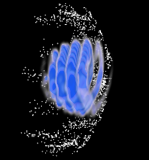
Now you can visualize the animation of the laser entering the window and pushing away the electrons, start experimenting with the many options of the selected representations, or with the colormaps and transfer functions.

Exporting data obtained in “AMcylindrical” geometry¶

In this geometry a cylindrical (x,r) grid is used for the fields, as explained its documentation. The axis r=0 corresponds to the propagation axis of the laser pulse. Furthermore, fields are defined through their cylindrical components, e.g. El, Er, Et instead of the Ex, Ey, Ez in "3Dcylindrical". Therefore, when using geometry="AMcylindrical" in the same input script you have used for this tutorial, some changes are made, in particular field and density profiles are defined on a (x,r) grid and the origins of the axes (in the profiles and the Probes) are shifted according to the different definition of their origins.

Change the geometry variable at the start of the namelist to have geometry="AMcylindrical" and run the simulation. The physical set-up is almost identical to the one simulated in "3Dcartesian" geometry, but for simplicity a Gaussian beam will be used for the Laser instead of a Laguerre-Gauss beam.

The commands to export macro-particle data from TrackParticles, except for the different axis origin, are identical to those used in the "3Dcartesian" case. This because the macro-particles (exactly as Probes) in "AMcylindrical" geometry are defined in the 3D space.

For the fields, you may in principle define 3D Probes in the namelist for the Cartesian components of the fields and export them to VTK adapting the previous commands, but we do not recommend this strategy. This way, the code would have to sample the Probe data in 3D during the simulation, creating a huge amount of data and slowing down your simulation, just to have data for visualization.

Instead, we recommend to export to vtk the Fields data defined in cylindrical geometry to the 3D cartesian space, though the argument build3d of the Fields available only in cylindrical geometry. For its synthax, see the Field documentation.

First, you need to specify an interval in the 3D cartesian space where you want have your VTK data. This interval is defined through a list, one for each axis x, y, z. Each list contains in order its lower and upper border and resolution in that direction. In this case, we can for example extract the data from the physical space that was simulated, so we can take the required values from the namelist. Afterwards, we export the Field data proportional to the laser intensity using build3d:

build3d_interval = [[0,S.namelist.Lx,S.namelist.dx]]
build3d_interval.append([-S.namelist.Ltrans,S.namelist.Ltrans,S.namelist.dtrans])
build3d_interval.append([-S.namelist.Ltrans,S.namelist.Ltrans,S.namelist.dtrans]])
E2 = S.Field.Field0("El**2+Er**2+Et**2",build3d = build3d_interval )

Note how we had to specify the cylindrical components of the fields. You do not have to export all the physical space or to use the same resolution specified in the namelist. For example, to reduce the amount of exported data you may choose to subsample the physical space with a coarser cell length.

Action: Try to define a Laguerre-Gauss beam profile in "AMcylindrical" geometry and simulate the same case you have simulated in "3Dcartesian" geometry. You will need some trigonometry to decompose the field in azimuthal modes, as described in the documentation.