
Patch arrangement
In some situations with slow particles dynamics, the dynamic load balancing may not be relevant to speed-up the simulation. Moreover, as it relies on a Hilbert curve, it may not be able to split intelligently the plasma in equal parts.
Typically, this happens when the plasma is contained in a thin slab. The Hilbert curve splitting is better replaced by a simple linearized splitting that divides the box in slabs of equal size.
The goal of this tutorial is to learn about these various arrangements of patches, and test them in realistic cases.
We recommand first to run the parallel computing tutorial.
Configuration
- Starting case :
To highlight the phenomenon and to simplify the discussion we propose to run on several MPI processes and only 1 thread per process.
Setting up the simulation
Set your simulation with 16 MPI processes, and only 1 thread per process. Typically:
export OMP_NUM_THREADS=1
mpirun -np 16 smilei radiation_pressure_acc_hilbert.py
Observe timers and the probe diagnostics results.
Note
Field diagnostics do not work with the alternative patch_arrangement
so we use Probe diagnostics instead.
Change the patch arrangement
Activate the dynamic load balancing to absorb synchronizations overhead
LoadBalancing(
    every = 20
)
A look at the plasma shape shows that, at initialization,
the plasma is located within a thin slab along the Y axis.
Then, it is pushed along the X axis.
We propose to enforce an arrangement of patches that splits
the plasma into slabs along X, so that each region owns an
equal share of the computational load.
You may add the following line in the bloc Main():
patch_arrangement = "linearized_YX",
We can imagine that splitting into slabs along Y would be a terrible option, because all the plasma will be contained in one process only. All other processes will need to wait and do nothing. You can still try it:
patch_arrangement = "linearized_XY",
You may want to stop the simulation before the end!
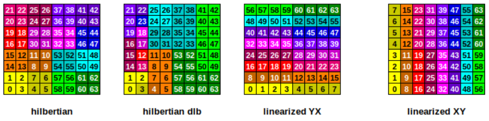
Fig. 1 Each numbered square represents a patch in an 8 x 8 patches configuration. Each color represents one of the 16 MPI processes. In this test case, the plasma is located in the 2nd column of the box. You can observe how the dynamic load balancing (dlb) makes a coarse splitting where there is no plasma.
Tuning the patch arrangement
In the situation above, there was a maximum of 8 patches in the Y direction, so that the plasma could not be split in more than 8 pieces. We would like to split it in 16 pieces to make sure that each of the 16 processes has something to work on. Unfortunatly the patch size, 75 x 125 cells, does not permit to split more in Y.
Study the following code, which slightly increases the spatial resolution in Y to get a number of cells in Y divisible per 16.
current_ncells_Y = Lsim[1] / (l0/resx)
target_ncells_Y = 1024.
target_cell_length_Y = (l0/resx*current_ncells_Y)/target_ncells_Y

Main(
    cell_length = [l0/resx,target_cell_length_Y],
)
It is available in the input file radiation_pressure_acc_linearized.py.
Run again the linearized_YX configuration: the higher resolution
leads to more particles, thus a slightly higher computation time.
You can now run the simulation with the 8 x 16 patches:
number_of_patches = [ 8, 16 ],
For a fair comparison, use this configuration with the hilbertian
arrangement (the default value of patch_arrangement).
In this mode, when the number of patches is not the same along all directions,
the Hilbert pattern is replicated in the larger direction (Y here).
This can be beneficial here.
Note
The paramater number_of_patches must be a power of 2
with the hilbertian arrangement. This is not required with the
linearized arrangement.