
Implementation
I. Introduction
Smilei is a C++ code that uses relatively simple C++ features for modularity and conveniency for non-advanced C++ users.
The repository is composed of the following directories:
Licence: contains code licence informationdoc: contains the Sphinx doc filessrc: contains all source fileshappi: contains the sources of the happi Python tool for visualizationbenchmarks: contains the benchmarks used by the validation process, these benchmarks are also examples for users.scripts: contains multiple tool scripts for compilation and morecompile_tools: contains scripts and machine files used by the makefile for compilation
tools: contains some additional programs for Smileivalidation: contains the python scripts used by the validation process
The source files directory is as well composed of several sub-directories to organise the .cpp and .h files by related thematics. The main is the file Smilei.cpp. There is always only one class definition per file and the file name corresponds to the class name.
The general implementation is later summarized in Fig. 80
II. General concept and vocabulary
This section presents some implicit notions to understand the philosophy of the code.
Notion of data container
Data containers are classes (or sometime just structures) used to store a specific type of data, often considered as raw data such as particles or fields. Some methods can be implemented in a data container for managing or accessing the data.
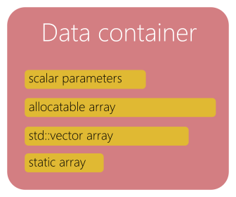
Fig. 71 Data container.
Notion of operators
An operator is a class that operates on input data to provide a processed information.
Input data can be parameters and data containers.
Output data can be processed data from data containers or updated data containers.
An operator is a class functor (overloading of the () ).
Sometime, operator provides additional methods called wrappers to provide different simplified or adapted interfaces.
An operator do not store data or temporarily.
for instance, the particle interpolation, push and protection are operators.
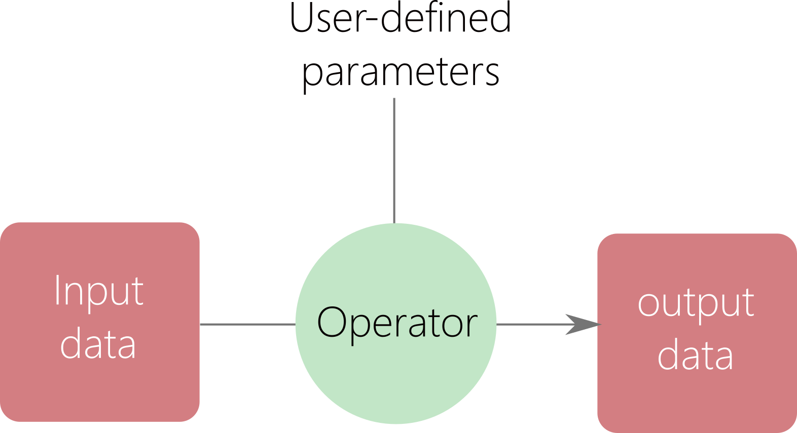
Fig. 72 Operator.
Notion of domain parts
Domain parts are classes that represents some specific levels of the domain decomposition.
They can be seen as high-level data container or container of data container.
They contain some methods to handle, manage and access the local data.
For instance, patches and Species are domain parts:
Speciescontains the particles.PatchcontainsSpeciesandFields.
Notion of factory
Some objects such as operators or data containers have several variations.
For this we use inheritance.
A base class is used for common parameters and methods and derived classes are used for all variations.
The factory uses user-defined input parameters to determine the right derived class to choose and initiate them as shown in Fig. 73.
For instance, there are several push operators implemented all derived from a base push class.
The push factory will determine the right one to use.
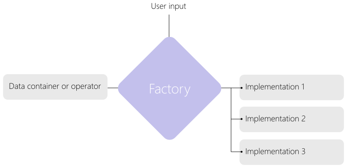
Fig. 73 Description of the factory concept.
Other
Some classes are used for specific actions in the code such as the initialization process.
III. Domain decomposition and parallelism
The simulation domain is divided multiple times following a succession of decomposition levels. The whole domain is the superimposition of different grids for each electromagnetic field component and macro-particles. Let us represent schematically the domain as an array of cells as in Fig. Fig. 74. Each cell contains a certain population of particles (that can differ from cell to cell).
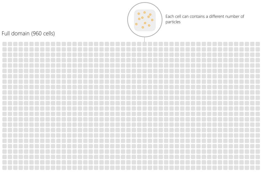
Fig. 74 Example of a full domain with 960 cells.
In smilei, the cells are first reorganized into small group so-called patches. The domain becomes a collection of patches as shown in Fig. 75.
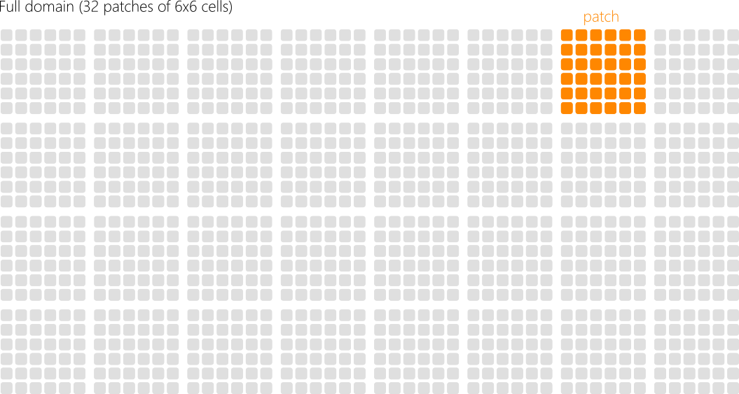
Fig. 75 The domain in Smilei is a collection of patches.
A patch is an independent piece of the whole simulation domain. It therefore owns the local electromagnetic grids and list of macro-particles. Electromagnetic grids have ghost cells that represent the information located in the neighboring patches (not shown in Fig. 75). All patches have the same spatial size .i.e. the same number of cells. The size of a patch is calculated so that all local field grids (ghost cells included) can fit in L2 cache.
Patches are then distributed among MPI processes in so-called MPI patch collections. The distribution can be ensured in an equal cartesian way or using a load balancing strategy based on the Hilbert curve.
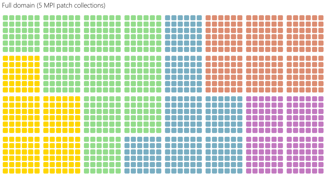
Fig. 76 Patches are then distributed among MPI processes in so-called MPI patch collections.
Inside MPI patch collection, OpenMP loop directives are used to distribute the computation of the patches among the available threads. Since each patch has a different number of particles, this approach enables a dynamic scheduling depending on the specified OpenMP scheduler. As shown in Fig. 80, a synchronization step is required to exchange grid ghost cells and particles traveling from patch to patch.
The patch granularity is used for:
creating more parallelism for OpenMP
enabling a load balancing capability through OpenMP scheduling
ensuring a good cache memory efficiency at L3 and L2 levels.
The patch is not the smaller decomposition grain-size. The patch can be decomposed into bins as shown in Fig. 77.
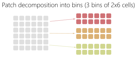
Fig. 77 Bin decomposition.
Contrary to patch, a bin is not an independent data structure with its own arrays. It represents a smaller portion of the patch grids through specific start and end indexes. For the macro-particles, a sorting algorithm is used to ensure that in the macro-particles located in the same bin are grouped and contiguous in memory.
Finally, the decomposition levels are summarized in Fig. 78.
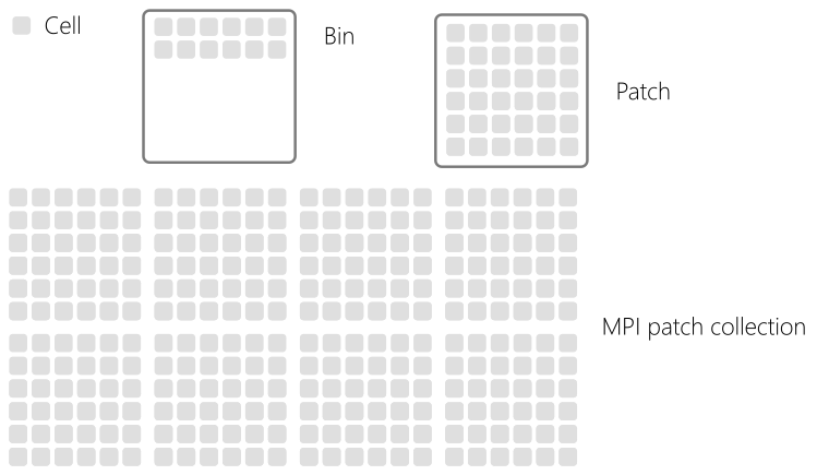
Fig. 78 Domain decomposition summary.
IV. Coding and community rules
Coding style rules
Line and indentation style
A line should be no more than 140 characters.
The code should not have some characters outside [0,127] in the ASCII table
There should be no more than 2 empty successive lines.
Only 1 statement per line is allowed.
An indentation block is only composed of 4 spaces, no tab is permitted.
If possible, keep trailing spaces in empty lines to respect indentation
For instance, this line is not correct:
a1 = b1 + c1*d1;
a2 = b2 + c2*d2;
and should be replaced by:
a1 = b1 + c1*d1;
a2 = b2 + c2*d2;
Variables
Variable names (public, protected, private, local) should be composed of lowercase and underscore between words.
The lowercase rule does not apply on acronyms and people names
For instance:
int number_of_elements;
int lignes_of_Smilei;
int age_of_GNU;
Classes
A class name starts with a capital letter
A capital letter is used between each word that composes the class name
No underscore
For instance:
class MyClassIsGreat
{
    public:
    int public_integer_;
    private:
    int private_integer_;
}
A class variable respects the rules of variables previously described.
A variable member has an underscore at the end of the name
Functions
Functions and member functions should start with a lowercase letter.
No underscore.
Each word starts with a capital letter.
For instance:
int myGreatFunction(...)
{
...
}
Names should be explicit as much as possible.
Avoid using shortened expression.
For instance:
void computeParticlePosition(...)
{
...
}
instead of:
void computePartPos(...)
{
...
}
If-statement
Any if-statement should have curly brackets.
For instance:
if( condition ) {
    a = b + c*d;
}
ERROR and OUTPUT management
Developers should use the dedicated error our output macro definition located in the file src/Tools.h.
ERROR: this function is the default one used to throw a SIGABRT error with a simple messages.
ERROR_NAMELIST: this function should be used for namelist error. It takes in argument a simple message and a link to the documentation. It throws as well a SIGABRT signal.
MESSAGE: this function should be used to output an information message (it uses std::cout).
DEBUG : should be used for debugging messages (for the so-called DEBUG mode)
WARNING : should be used to thrown a warning. A warning alerts the users of a possible issue or to be careful with some parameters without stopping the program.
V. Data structures and main classes
This section describes the main classes and the tree-like smilei data structure. The whole picture is shown in Fig. 79.
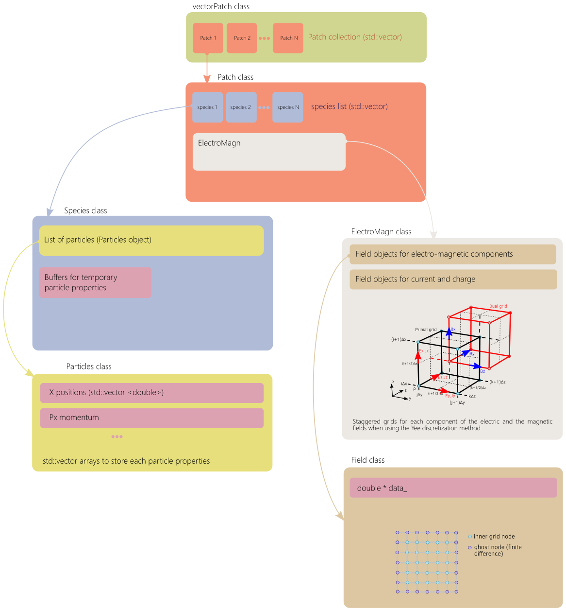
Fig. 79 General of the main tree-like data structure of Smilei.
Class VectorPatch
The class VectorPatch represents the MPI Patch collection described above and is the highest structure level.
The class description (vectorPatch.h and vectorPatch.cpp) is located in the directory src/Patch.
Among the data components stored in this class, one of the most important is the list of patches.
By definition, each MPI process has therefore only one declared vectorPatch object.
-
class VectorPatch
-
List of patches located in this MPI patch collection.
The class VectorPatch contains the methods directly called in the PIC time loop in smilei.cpp.
Class Patch
The class Patch is an advanced data container that represents a single patch.
The base class description (Patch.h and Patch.cpp) is located in the directory src/Patch.
From this base class can be derived several versions (marked as final) depending on the geometry dimension:
Patch1DPatch2DPatch3DPatchAMfor the AM geometry
The class Patch has a list of object Species called vecSpecies.
-
class Patch
-
List of species in the patch
-
ElectroMagn *EMfields
Electromagnetic fields and densities (E, B, J, rho) of the current Patch
-
ElectroMagn *EMfields
class Species
The class Species is an advanced data container that represents a single species.
The base class description (Species.h and Species.cpp) is located in the directory src/Species.
From this base class can be derived several versions (marked as final):
SpeciesNormSpeciesNormVSpeciesVSpeciesVAdaptiveSpeciesVAdaptiveMixedSort
The correct species object is initialized using the species factory implemented in the file speciesFactory.h.
The class Species owns the particles through the object particles of class Particles*.
class Particles
The class Particles is a data container that contains the particle properties.
The base class description (Particles.h and Particles.cpp) is located in the directory src/Particles.
It contains several arrays storing the particles properties such as the positions, momenta, weight and others.
-
class Particles
-
std::vector<std::vector<double>> Position
Array containing the particle position
-
std::vector<std::vector<double>> Momentum
Array containing the particle moments
-
std::vector<double> Weight
Containing the particle weight: equivalent to a charge density
-
std::vector<double> Chi
containing the particle quantum parameter
-
std::vector<double> Tau
Incremental optical depth for the Monte-Carlo process
-
std::vector<short> Charge
Charge state of the particle (multiples of e>0)
-
std::vector<uint64_t> Id
Id of the particle
-
std::vector<int> cell_keys
cell_keys of the particle
-
std::vector<std::vector<double>> Position
Many of the methods implemented in Particles are used to access or manage the data.
class ElectroMagn
The class ElectroMagn is a high-level data container that contains the electromagnetic fields and currents.
The base class description (ElectroMagn.h and ElectroMagn.cpp) is located in the directory src/ElectroMagn.
From this base class can be derived several versions (marked as final) based on the dimension:
ElectroMagn1DElectroMagn2DElectroMagn3DElectroMagnAM
The correct final class is determined using the factory ElectroMagnFactory.h.
class Field
The class Field is a data-container that represent a field grid for a given component.
The base class description (Field.h and Field.cpp) is located in the directory src/Field.
It contains a linearized allocatable array to store all grid nodes whatever the dimension.
-
class Field
-
double *data_
pointer to the linearized field array
From this base class can be derived several versions (marked as
final) based on the dimension:Field1DField2DField3D
-
double *data_
The correct final class is determined using the factory FieldFactory.h.
Smilei MPI
The class SmileiMPI is a specific class that contains interfaces and advanced methods for the custom and adapted use of MPI within Smilei.
The base class description (SmileiMPI.h and SmileiMPI.cpp) is located in the directory src/SmileiMPI.
-
class SmileiMPI
VI. The Smilei PIC loop implementation
The initialization and the main loop are explicitely done in the main file Smilei.cpp.
The time loop is schematically described in Fig. 80.
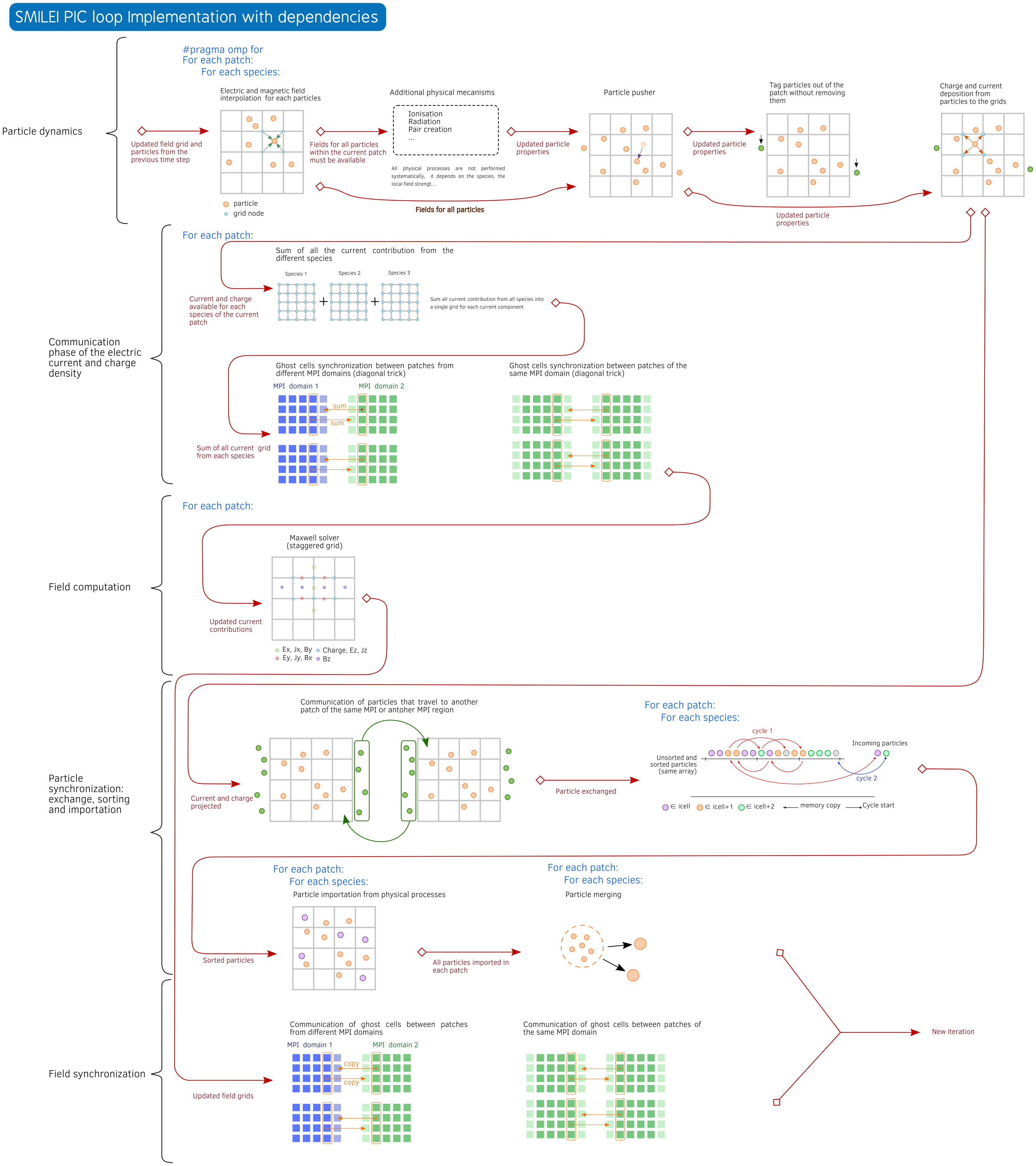
Fig. 80 Smilei main loop implementation (click on the figure for more details).
The time loop is explicitely written step by step in the main
file Smilei.cpp thought calls to different vecPatches methods.
Patch reconfiguration: if adaptive vectorization is activated, then the patch may be reconfigured for scalar or vectorized mode.
vecPatches.reconfiguration( params, timers, itime );
Collision: particle collisions are performed before the particle dynamics part
vecPatches.applyBinaryProcesses( params, itime, timers );
Relativistic poisson solver: …
vecPatches.runRelativisticModule( time_prim, params, &smpi, timers );
Charge: reset global charge and currents densities to zero and computes rho old before moving particles
vecPatches.computeCharge(true);
Particle dynamics: this step processes the full particle dynamics including field interpolation, advanced physical operators (radiation, ionization…), boundary condition pre-processing and projection
vecPatches.dynamics( params, &smpi, simWindow, radiation_tables_,
                                 MultiphotonBreitWheelerTables,
                                 time_dual, timers, itime );
Envelope module: …
vecPatches.runEnvelopeModule( params, &smpi, simWindow, time_dual, timers, itime );
Sum of currents and densities: current et charge reduction from different species and perform the synchronization step with communication
vecPatches.sumDensities( params, time_dual, timers, itime, simWindow, &smpi );
Maganement of the antenna: apply currents from antennas
vecPatches.applyAntennas( time_dual );
Maxwell solvers: solve Maxwell
vecPatches.solveMaxwell( params, simWindow, itime, time_dual, timers, &smpi );
Particle communication: finalize particle exchanges and sort particles
vecPatches.finalizeExchParticlesAndSort( params, &smpi, simWindow,
                                             time_dual, timers, itime );
Particle merging: merging process for particles (still experimental)
vecPatches.mergeParticles(params, time_dual,timers, itime );
Particle injection: injection of particles from the boundaries
vecPatches.injectParticlesFromBoundaries(params, timers, itime );
Cleaning: Clean buffers and resize arrays
vecPatches.cleanParticlesOverhead(params, timers, itime );
Field synchronization: Finalize field synchronization and exchanges
vecPatches.finalizeSyncAndBCFields( params, &smpi, simWindow, time_dual, timers, itime );
Diagnostics: call the various diagnostics
vecPatches.runAllDiags( params, &smpi, itime, timers, simWindow );
Moving window: manage the shift of the moving window
1timers.movWindow.restart();
2simWindow->shift( vecPatches, &smpi, params, itime, time_dual, region );
3
4if (itime == simWindow->getAdditionalShiftsIteration() ) {
5    int adjust = simWindow->isMoving(time_dual)?0:1;
6    for (unsigned int n=0;n < simWindow->getNumberOfAdditionalShifts()-adjust; n++)
7        simWindow->shift( vecPatches, &smpi, params, itime, time_dual, region );
8}
9timers.movWindow.update();
Checkpointing: manage the checkoints
checkpoint.dump( vecPatches, region, itime, &smpi, simWindow, params );
Particle Dynamics
The particle dynamics is the large step in the time loop that performs the particle movement computation:
Field interpolation
Radiation loss
Ionization
Pair creation
Push
Detection of leaving particles at patch boundaries
Charge and current projection
This step is performed in the method vecPatches::dynamics.
We first loop on the patches and then the species of
each patch ipatch: (*this )( ipatch )->vecSpecies.size().
For each species, the method Species::dynamics is called to perform the
dynamic step of the respective particles.
The OpenMP parallelism is explicitly applied in vecPatches::dynamics on the patch loop as shown
in the following pieces of code.
 1#pragma omp for schedule(runtime)
 2for( unsigned int ipatch=0 ; ipatch<this->size() ; ipatch++ ) {
 3
 4    // ...
 5
 6    for( unsigned int ispec=0 ; ispec<( *this )( ipatch )->vecSpecies.size() ; ispec++ ) {
 7        Species *spec = species( ipatch, ispec );
 8
 9        // ....
10
11        spec->Species::dynamics( time_dual, ispec,
12                                 emfields( ipatch ),
13                                 params, diag_flag, partwalls( ipatch ),
14                                 ( *this )( ipatch ), smpi,
15                                 RadiationTables,
16                                 MultiphotonBreitWheelerTables );
17
18        // ...
19
20    }
21}
Pusher
The pusher is the operator that moves the macro-particles using the equations of movement.
The operator implementation is
located in the directory src/Pusher.
The base class is Pusher implemented in Pusher.h and Pusher.cpp.
From this base class can be derived several versions (marked as final):
PusherBoris: pusher of BorisPusherBorisNR: non-relativistic Boris pusherPusherBorisV: vectorized Boris pusherPusherVay: pusher of J. L. VayPusherHigueraCary: pusher of Higuera and CaryPusherPhoton: pusher of photons (ballistic movement)
A factory called PusherFactory is used to select the requested pusher for each patch and each species.
Note
Whatever the mode on CPU, the pusher is always vectorized.
Boris pusher for CPU
The pusher implementation is one of the most simple algorithm of the PIC loop.
In the initialization part of the functor, we use pointers to simplify the access to the different arrays.
The core of the pusher is then composed of a single vectorized loop (omp simd) over a group of macro-particles.
 1        is_device_ptr( /* tofrom: */                                          \
 2                       momentum_x /* [istart:particle_number] */,             \
 3                       momentum_y /* [istart:particle_number] */,             \
 4                       momentum_z /* [istart:particle_number] */,             \
 5                       position_x /* [istart:particle_number] */,             \
 6                       position_y /* [istart:particle_number] */,             \
 7                       position_z /* [istart:particle_number] */ )
 8    #pragma omp teams distribute parallel for
 9#elif defined(SMILEI_ACCELERATOR_GPU_OACC)
10    const int istart_offset   = istart - ipart_buffer_offset;
11    const int particle_number = iend - istart;
12
13    #pragma acc parallel present(Ex [0:nparts],    \
14                                 Ey [0:nparts],    \
15                                 Ez [0:nparts],    \
16                                 Bx [0:nparts],    \
17                                 By [0:nparts],    \
18                                 Bz [0:nparts],    \
19                                 invgf [0:nparts]) \
20        deviceptr(position_x,                                           \
21                  position_y,                                           \
22                  position_z,                                           \
23                  momentum_x,                                           \
24                  momentum_y,                                           \
25                  momentum_z,                                           \
26                  charge)
27    #pragma acc loop gang worker vector
28#else
29    #pragma omp simd
30#endif
31    for( int ipart=istart ; ipart<iend; ipart++ ) {
32
33        const int ipart2 = ipart - ipart_buffer_offset;
34
35        const double charge_over_mass_dts2 = ( double )( charge[ipart] )*one_over_mass_*dts2;
36
37        // init Half-acceleration in the electric field
38        double pxsm = charge_over_mass_dts2*( Ex[ipart2] );
39        double pysm = charge_over_mass_dts2*( Ey[ipart2] );
40        double pzsm = charge_over_mass_dts2*( Ez[ipart2] );
41
42        //(*this)(particles, ipart, (*Epart)[ipart], (*Bpart)[ipart] , (*invgf)[ipart]);
43        const double umx = momentum_x[ipart] + pxsm;
44        const double umy = momentum_y[ipart] + pysm;
45        const double umz = momentum_z[ipart] + pzsm;
46
47        // Rotation in the magnetic field
Boris pusher for GPU
On GPU, the omp simd directives is simply changed for the #pragma acc loop gang worker vector.
The macro-particles are distributed on the GPU threads (vector level).
Nonlinear Inverse Compton radiation operator
The physical details of this module are given in the page High-energy photon emission & radiation reaction.
The implementation for this operator and the related files are located in the directory
src/Radiation.
The base class used to derive the different versions of this operator is called Radiation
and is implemented in the files Radiation.h and Radiation.cpp.
A factory called RadiationFactory is used to select the requested radiation model for each patch and species.
The different radiation model implementation details are given in the following sections.
Landau-Lifshift
The derived class that correspponds to the Landau-Lifshift model is called RadiationLandauLifshitz and
is implemented in the corresponding files.
The implementation is relatively simple and is similar to what is done in the Pusher
since this radiation model is an extension of the classical particle push.
 1    // _______________________________________________________________
 2    // Computation
 3
 4    #ifndef SMILEI_ACCELERATOR_GPU_OACC
 5        #pragma omp simd aligned(rad_norm_energy:64)
 6    #else
 7        int np = iend-istart;
 8        #pragma acc parallel \
 9            present(Ex[istart:np],Ey[istart:np],Ez[istart:np],\
10            Bx[istart:np],By[istart:np],Bz[istart:np]) \
11            deviceptr(momentum_x,momentum_y,momentum_z,charge,weight,chi) \
12            reduction(+:radiated_energy_loc)
13    {
14        #pragma acc loop reduction(+:radiated_energy_loc) gang worker vector private(rad_norm_energy)
15    #endif
16    for( int ipart=istart ; ipart<iend; ipart++ ) {
17
18        // charge / m^2
19        const double charge_over_mass_square = ( double )( charge[ipart] )*one_over_mass_square;
20
21        // Gamma
22        const double gamma = sqrt( 1.0 + momentum_x[ipart]*momentum_x[ipart]
23                      + momentum_y[ipart]*momentum_y[ipart]
24                      + momentum_z[ipart]*momentum_z[ipart] );
25
26        // Computation of the Lorentz invariant quantum parameter
27        const double particle_chi = Radiation::computeParticleChi( charge_over_mass_square,
28                       momentum_x[ipart], momentum_y[ipart], momentum_z[ipart],
29                       gamma,
30                       Ex[ipart-ipart_ref], Ey[ipart-ipart_ref], Ez[ipart-ipart_ref] ,
31                       Bx[ipart-ipart_ref], By[ipart-ipart_ref], Bz[ipart-ipart_ref] );
32
33        // Effect on the momentum
34        if( gamma > 1.1 && particle_chi >= minimum_chi_continuous ) {
35
36            // Radiated energy during the time step
37            const double temp =
38                radiation_tables.getClassicalRadiatedEnergy( particle_chi, dt_ ) * gamma / ( gamma*gamma-1. );
It is composed of a vectorized loop on a group of particles using the istart and iend indexes
given as argument parameters to perform the following steps:
Commputation of the particle Lorentz factor
Commputation of the particle quantum parameter (
particle_chi)Update of the momentum: we use the function
getClassicalRadiatedEnergyimplemented in the classRadiationTablesto get the classical radiated energy for the given particle.Computation of the radiated energy: this energy is first stored per particle in the local array
rad_norm_energy
The second loop performs a vectorized reduction of the radiated energy for the current thread.
1            momentum_z[ipart] -= temp*momentum_z[ipart];
2
3    // _______________________________________________________________
4    // Computation of the thread radiated energy
5
6#ifndef SMILEI_ACCELERATOR_GPU_OACC
The third vectorized loop compute again the quantum parameters based on the new momentum
and this time the result is stored in the dedicated array chi[ipart] to be used in
the following part of the time step.
 1                                              + momentum_z[ipart]*momentum_z[ipart] );
 2        }
 3    }
 4
 5    #pragma omp simd reduction(+:radiated_energy_loc)
 6    for( int ipart=0 ; ipart<iend-istart; ipart++ ) {
 7        radiated_energy_loc += weight[ipart]*rad_norm_energy[ipart] ;
 8    }
 9#else
10            radiated_energy_loc += weight[ipart]*(gamma - std::sqrt( 1.0
11                                              + momentum_x[ipart]*momentum_x[ipart]
12                                              + momentum_y[ipart]*momentum_y[ipart]
13                                              + momentum_z[ipart]*momentum_z[ipart] ));
14#endif
15
16
17    // _______________________________________________________________
Corrected Landau-Lifshift
The derived class that correspponds to the corrected Landau-Lifshift model is called RadiationCorrLandauLifshitz and
is implemented in the corresponding files.
Niel
The derived class that correspponds to the Nield model is called RadiationNiel and
is implemented in the corresponding files.
Monte-Carlo
The derived class that correspponds to the Monte-Carlo model is called RadiationMonteCarlo and
is implemented in the corresponding files.
Radiation Tables
The class RadiationTables is used to store and manage the different tabulated functions
used by some of the radiation models.
Radiation Tools
The class RadiationTools contains some function tools for the radiation.
Some methods provide function fit from tabulated values obtained numerically.
Particle Event Tracing
To visualize the scheduling of operations, an macro-particle
event tracing diagnostic saves the time when each OpenMP thread executes one of these
operations and the involved thread’s number. The PIC operators (and the advanced ones like
Ionization, Radiation) acting on each ipatch-ispec-ibin combination are
included in this diagnostic.
This way, the macro-particle operations executed by each OpenMP thread in each
MPI process can be visualized. The information of which bin, Species, patch
is involved is not stored, since it would be difficult to visualize this level of
detail. However it can be added to this diagnostic in principle.
This visualization becomes clearer when a small number of patches, Species,
bins is used. In other cases the plot may become unreadable.