Exercises
Tips for the exercises
Organization: you will soon arrive to exercises that ask to run one or more simulations. To avoid overwriting previous simulation data, and to avoid forgetting where previous simulations were run (especially if you want to recheck your answers), create a new folder for each simulation, giving it a meaningful name, and keeping your data space organized. If it helps, you may also take notes on the path of the folders to remember where each simulation was run.
Read the namelist: the comments in the namelist and the defined variables contain also useful information for exercises.
Read again the practical presentation: some of the explained concepts may help you during the exercises.
Parallelizing the simulations: While working on a supercomputer, normally to launch a new simulation you don't have to wait for the last one you have launched to be complete. If no computing resources are available yet, the newly launched simulations will wait in the queue.
Questions? Doubts? Ask the instructor!
Exploring the input namelist
To run a simulation, you need to specify the phenomena it will describe and
the numerical parameters to study your case, e.g. the resolution, the integration timestep, the grid size,
in an input file, in this case called InputNamelist.py.
In the next few exercises we will understand the basic set-up of a simulation described this file.
One of the first variables we define in this simulation is the lambda0, i.e. the laser carrier frequency
\(\lambda_0\).
Exercise 1
Assuming \(\lambda_0=0.8 \mu m\) (a Ti:Sa laser system), what is the value of the critical density \(n_c\)?
What is the value of the reference electric field \(E_0=(2\pi m_e c^2)/(e\lambda_0)\)?
This choice of \(\lambda_0\) will be used throughout all subsequent exercises.
Hint: Some lines at the start of the InputNamelist.py file can help you in the calculations.
The InputNamelist.py file starts with the definition of physical constants and units,
mesh points, integration timestep, etc.
Some of these parameters are inserted in the first block of the simulation, called Main block.
Others may be useful for conversions between units or to define other variables in the file.
In the Main block, you will also find the geometry of the simulation, which is AMcylindrical.
The grid where Maxwell's equations are solved is defined on a cylindrical space and with cylindrical coordinates x, r, but the particles move in the 3D space
x, y, z (See Fig. 1).
The use of cylindrical coordinates with cylindrical symmetry enables quick
simulations with accuracy comparable to 3D simulations.
Note a block called MovingWindow in the InputNamelist.py.
In the physical case being considered, a laser pulse with duration of tens
of femtoseconds propagating along the positive x direction is simulated.
We are only interested in phenomena near the laser pulse
(within tens of microns), like plasma wave excitation, so a Moving Window is defined,
which emulates a camera moving at the speed
we want, along the positive x direction.
In this physical case, the moving window speed is set to c to follow the laser. As a result,
the laser pulse is almost immobile in the simulation window.
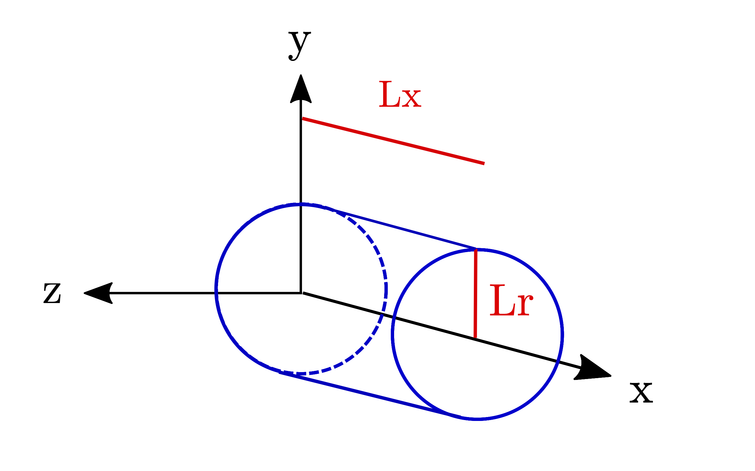
Fig. 1 Reference axes of the simulation. The simulation window corresponds to the cylinder with radius Lr and length Lx.
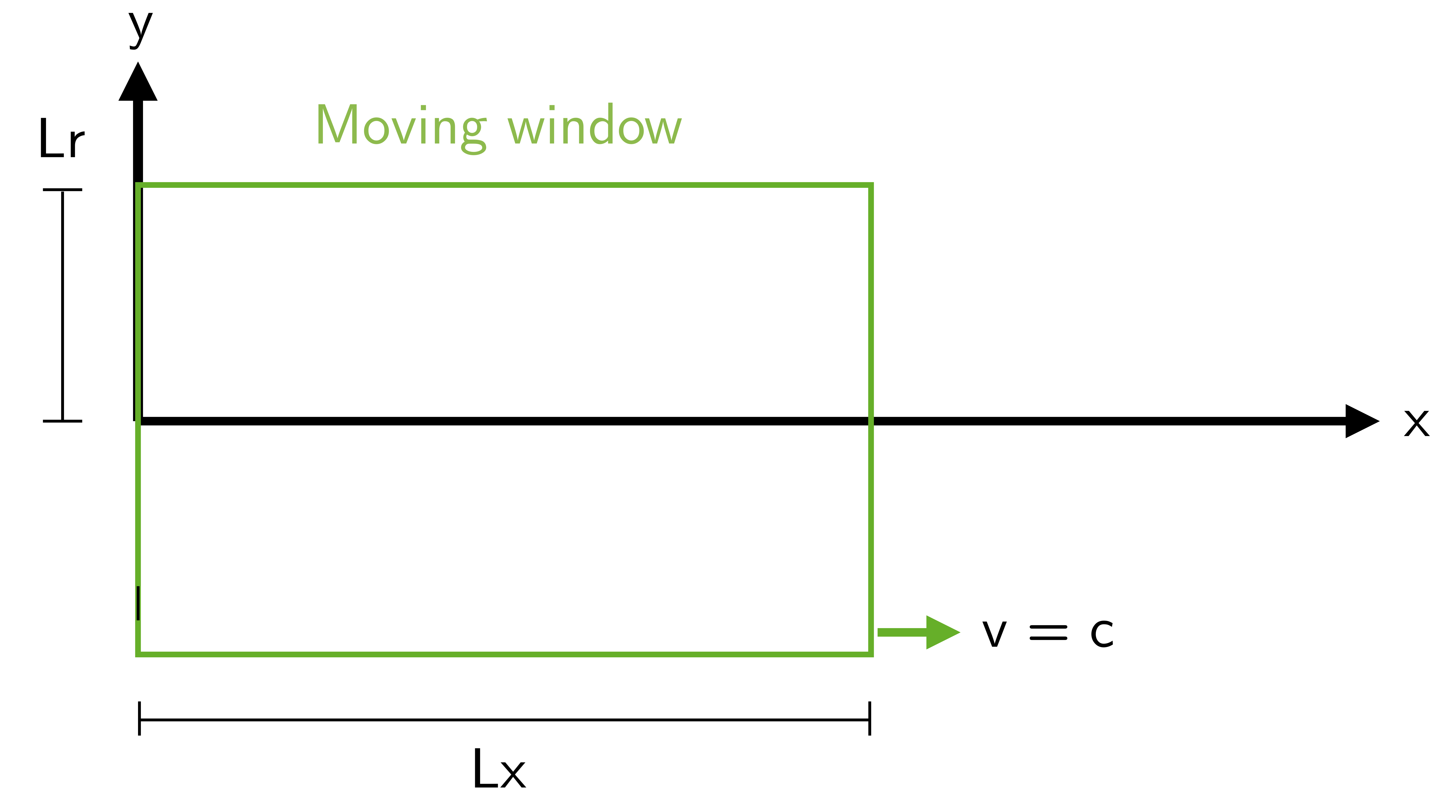
Fig. 2 Set-up of the simulation moving window at time t=0 (not to scale).
The physical elements inside the window are not shown.
Exercise 2
What are the longitudinal size Lx and radial size Lr of the simulation window?
How many mesh points nx and nr are used in the longitudinal and radial directions?
What is the resolution dx and dr in the longitudinal and radial directions?
See Figures 1 and, 2 for reference, and find these lengths in the InputNamelist.py.
Note: executing the namelist lines defining the variables Lx and Lr will give their values in normalized units, not in physical units.
At the end of the InputNamelist.py file,
there are blocks starting with the word Diag.
These blocks are for the diagnostics/outputs of the code.
The first Diag is a DiagProbe defined on a line
(so a 1D diagnostic), on the propagation axis of the laser (the x axis).
This diagnostic returns the value of some physical fields
along that axis. We call this probe Probe0 (the 0 because
it is the first Probe in the namelist). The second diagnostic block is
a DiagProbe defined on the plane xy (so a 2D diagnostic).
This is the second probe of the namelist, so it is called Probe1.
Laser pulse in vacuum
Everything is ready to run your first simulation.
We will start adding a laser pulse propagating in vacuum, along the positive x direction.
Action: at the start of the InputNamelist.py file, launch the simulation after ensuring that the desired physical case is selected:
selected_case = "laser_in_vacuum"
For the physical cases we will simulate with a laser pulse, a code block defines a laser pulse in the simulation with a transverse field based on the definition of a Gaussian Beam [Siegman], with a carrier wavelength \(\lambda_0 = 0.8 \mu m\).
The considered pulse also has Gaussian temporal profile, whose FWHM length is much larger
than the laser carrier wavelength \(\lambda_0\), defined in the variable lambda0 (see Fig. 3).
The laser transverse electric field is linearly polarized in the y direction.
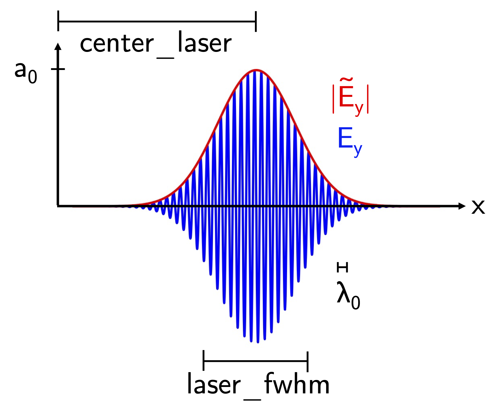
Fig. 3 Definition of the laser parameters (not to scale). In blue, the normalized transverse electric field of the laser, in red the absolute value of its complex envelope. All quantities are in normalized units (e.g. \(\lambda_0/2\pi\) for the lengths, \(m_e\omega_0c/e\) for the fields).
The simulation for this physical case includes a moving window and a laser pulse, as in Fig. 4.
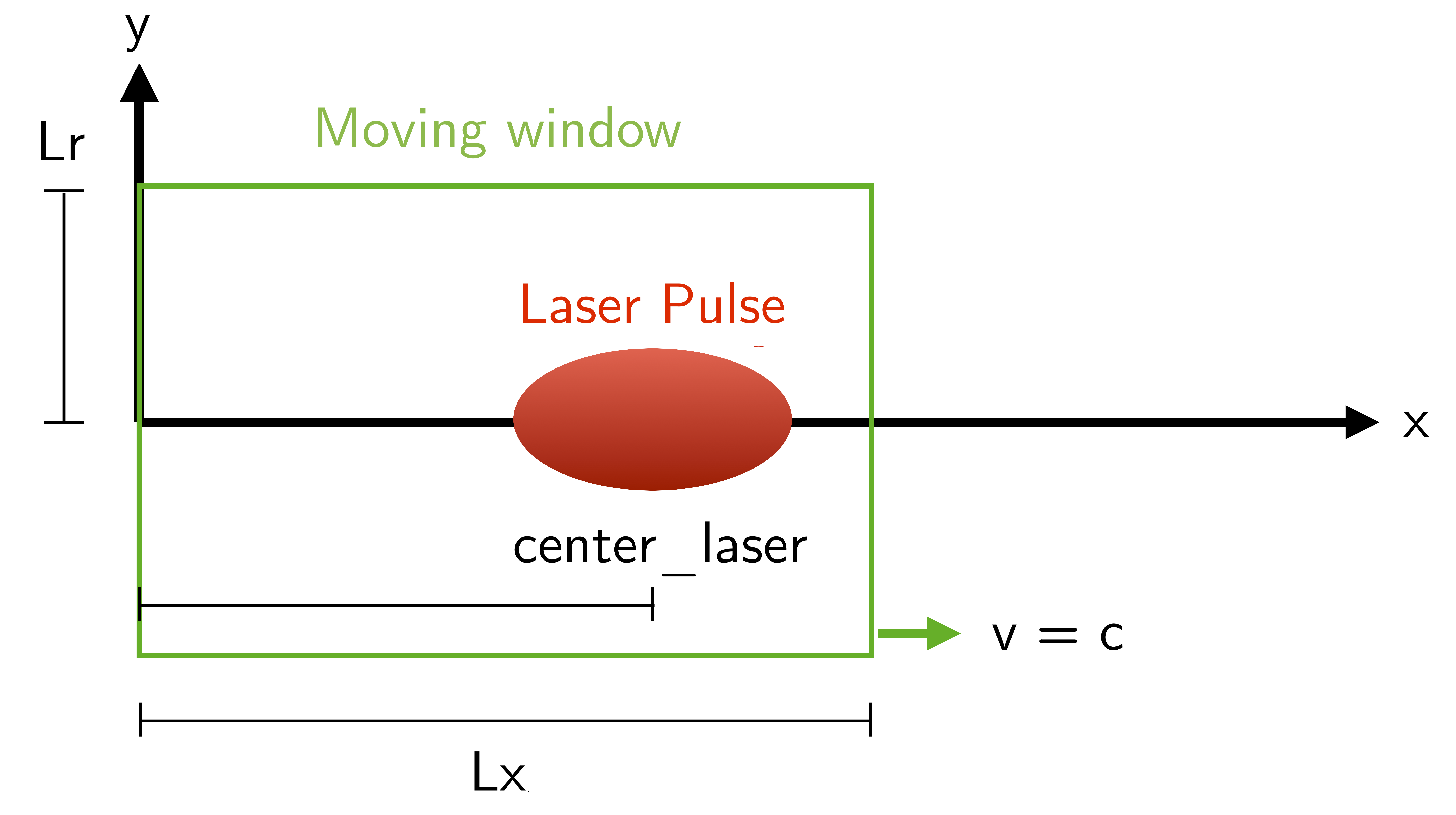
Fig. 4 Set-up of the simulation moving window at time t=0 (not to scale).
Note: an envelope model is used to describe the laser pulse, as described in [Massimo].
Therefore, the laser field and the electromagnetic fields it will excite in the plasma
will not show the high frequency oscillations as in the blue line of Fig. 3.
The absolute value of the complex envelope of the laser transverse electric field is contained in the field Env_E_abs.
Exercise 3
Find the laser pulse parameters in the InputNamelist.py.
What are the waist size, FWHM duration in field, and FWHM duration in intensity of the laser pulse?
Normally the duration of laser pulses is experimentally characterized by its FWHM in intensity, but the Laser... block in the namelist
defines a quantity associated with the laser field.
Hint: for a Gaussian temporal profile, the FWHM duration in intensity is \(1./\sqrt{2}\) times the FWHM duration in field.
In the simulation window, what is the x_center_laser coordinate of the center of the laser pulse at the start of the simulation?
Where is the focal plane of the laser pulse (variable x_focus_laser)?
Note: executing the namelist lines defining these variables will give their values in normalized units, not in physical units.
Exercise 4
The normalized laser peak field is given by \(a_0 = eE/m_e\omega_0c\), where \(E\) is the laser electric field peak and \(\omega_0 = 2\pi c/\lambda_0\) is the laser central frequency (\(\lambda_0 = 0.8 \mu m\).)
Using the laser \(a_0\) set in the namelist for the calculations, what is the laser peak averaged intensity \(I = c\varepsilon_0 |E|^2/2\) of the laser pulse?
Hint: the input namelist contains the physical quantities that you may need for the conversions.
Action: When the simulation is completed (the word END should appear in the log file), open IPython with the command ipython.
Then, you can check the initial position of the laser through the commands:
import happi; S = happi.Open()
S.Probe.Probe0("Env_E_abs",units=["um","fs","TV/m"],timesteps=0).plot( figure=1, xlabel="x [um]")
S.Probe.Probe1("Env_E_abs",units=["um","fs","TV/m"],timesteps=0).plot( figure=2, xlabel="x [um]",ylabel="y [um]")
Probe0 is a 1D diagnostic defined on the laser propagation axis, while Probe1 is a
2D diagnostic defined on the plane \(xy\). Note that in the commands we have specified
timesteps=0 to see the laser pulse at the start of the simulation.
Check that the initial laser position that you are seeing is the same specified in the input namelist. Remember that the laser pulse is modeled through its envelope, so you can not see its high frequency oscillations with wavelength \(\lambda_0\).
We can study the laser diffraction in vacuum. To see the evolution of the laser, use:
S.Probe.Probe1("Env_E_abs",units=["um","fs","TV/m"]).slide( figure=3, xlabel="x [um]",ylabel="y [um]" )
You can move the horizontal time bar to see the snapshots at different iterations. Note that the Moving Window makes the laser seem immobile in the simulation, but it is moving at speed c in vacuum, and the Moving Window is following it with the same speed.
If you do not specify a vmax value (the colorbar maximum) in the previous command,
happi will change it at each iteration. To better see the laser diffraction,
try to specify a colormap maximum with vmax. For example:
S.Probe.Probe1("Env_E_abs",units=["um","fs","TV/m"]).slide( figure=3,vmax=2., xlabel="x [um]",ylabel="y [um]" )
Exercise 5
In the this exercise we will check that the Gaussian laser pulse diffracts following the theory for a Gaussian beam [Siegman]: \(w(x) = w_0\sqrt{1 + (x-x_{focus})^2/x^2_R }\), where \(w_0\) is the laser waist size at the focal plane position \(x_{focus}\), \(w(x)\) the laser waist size at propagation distance \(x\), \(x_R\) is the Rayleigh length \(x_R = \pi w_0^2/\lambda_0\).
In our case, what is the theoretical Rayleigh length \(x_R\)?
Action: Use the script Laser_waist_theory_vs_Smilei.py
to compare the analytical diffraction law for \(w(x)\) and the laser waist extracted from your Particle-in-Cell (PIC) simulations results.
Copy the script in the simulation folder or call the script from that folder.
The script loads the field quantities on the plane xy, then loops over the iterations available in output
and computes the laser pulse waist \(w(x)\) along that plane as
where \(\tilde{A}\) is the complex envelope of the laser transverse vector potential.
After this calculation, the simulated waist is compared to the corresponding analytical value.
Run the script (from IPython use %run Laser_waist_theory_vs_Smilei.py)
to plot the comparison and include the image in your answers.
Exercise 6 (advanced)
We are using boundary conditions called Perfectly Matched Layers to prevent unphysical field reflections at the borders of the simulation window, but no numerical boundary condition can perfectly absorb a laser which does not fit in the window from the start. All PIC codes have the habit of running without telling you if something unphysical happens, so we often need to check if unphysical phenomena are occurring in the simulation.
Action: in another folder, run the same simulation, but with a smaller simulation window.
Change the variable nr to 64 at the start of the namelist, to simulate what would have happened if we had
chosen a window size too small compared to the laser transverse size.
What is the resulting transverse size Lr of the new window?
Use again the script of the previous exercise to compare the results with the theory and include the image in your answers.
How do you explain the results?
Hint: Use again the command:
S.Probe.Probe1("Env_E_abs",units=["um","fs","TV/m"]).slide( figure=3,vmax=2., xlabel="x [um]",ylabel="y [um]" )
and include a clarifying image in your answer.
In the following exercises, use again the original value of nr.
Laser wakefield excitation
Now we will add a preionized hydrogen plasma to excite plasma waves in the wake of the laser pulse. The laser pulse is considered intense enough to assume that the hydrogen gas was already ionized, much before the arrival of the laser pulse peak (see the laser intensity computed in Exercise 3).
Action: at the start of the InputNamelist.py file, change the variable selected_case to:
selected_case = "laser_wakefield_excitation"
This activates an additional block that defines a particle Species
in the simulation, whose name is plasmaelectrons. Note the normalized mass
and normalized charge of these particles defined in this block (1.0 and -1.0 respectively).
Since the normalizing mass and charge are the electron mass and the unit charge,
we know that these particles are electrons.
After a short linear ramp, the plasma density profile
is uniform for one millimetre in the x direction and within a distance Radius_plasma=30 \(μm\)
from the laser's propagation axis.
Therefore, now the simulation includes a moving window, a laser pulse (modeled by its complex envelope) and electron plasma, as represented in Fig. 5.
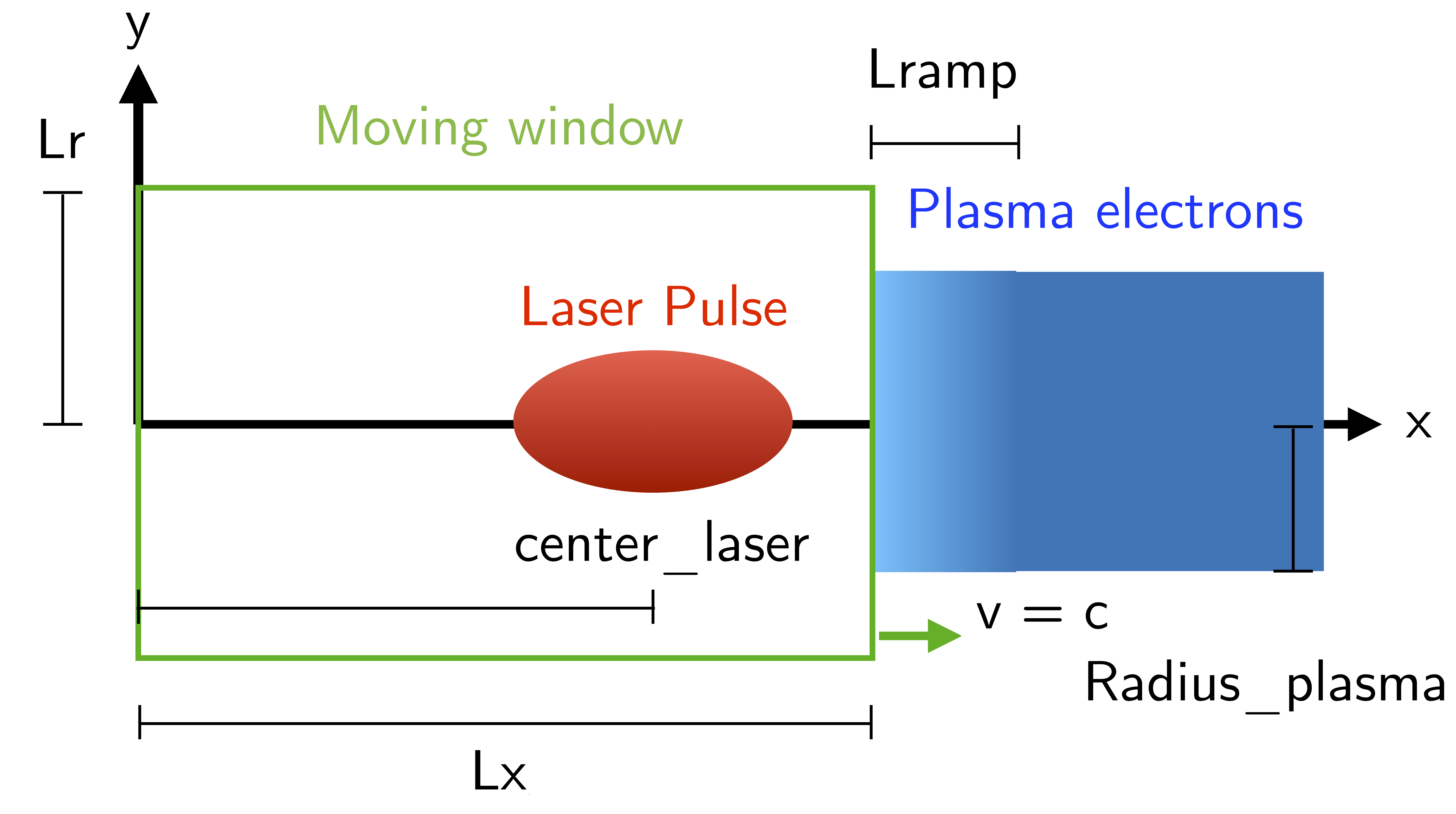
Fig. 5 Simulation Setup at the start of the simulation(s) in this Section (not to scale).
Exercise 7
As you can see, the plasma density has a value \(n_0 = 10^{18} electrons/cm^{3}\).
What is the ratio between the plasma density and the critical density (computed for Exercise 1)? Pay attention to the units!
Is it an underdense or overdense plasma?
The variable particles_per_cell of the Species block with name="plasmaelectrons"
contains the number of macro-particles per cell of that Species. Using this number, and the total number of mesh cells
in the simulation window (see Exercise 2), can you estimate how many macro-particles
would be simulated in the simulation window if it was filled by uniformly distributed macro-particles?
This simulation is uses a cylindrical grid, simulating only the half-plane \(r>0\).
Using the same particles_per_cell and again a simulation window uniformly filled of macro-particles,
how many macro-particles would be contained in a 3D simulation window with the same resolution of this namelist
in the longitudinal and transverse directions, and with size Lx, 2*Lr, and 2*Lr
in the x, y and z directions?
(This answer may give a clue on why simulations in cylindrical geometry are generally faster ...)
As we did with in Exercise 6 for the laser pulse in vacuum,
the first step to check our results is to verify that the plasma behaves as predicted by
the analytical theory. If we reduce the laser pulse a0 to 0.01,
the laser pulse satisfy the conditions for the applicability of the
1D linear theory of plasma wave excitation.
Exercise 8
The analytical 1D linear theory (which can be applied in our case for \(a_0 \ll 1\)) predicts the formation of a sinusoidal wave at plasma frequency \(\omega_p^2 = e^2n_0/m_e\varepsilon_0\) behind the laser, where \(n_0\) is the plasma density.
Action: Launch the simulation with \(a_0 = 0.01\) (you will need to change this variable in the InputNamelist.py).
Study the evolution of the electric field Ex with the diagnostics Probe0 and Probe1.
You can use the same plot commands of the previous section, but applied to Ex instead of Env_E_abs,
for example with
import happi; S=happi.Open()
S.Probe.Probe0("Ex",units=["um","fs","GV/m"]).slide( figure=3, xlabel="x [um]" );
S.Probe.Probe1("Ex",units=["um","fs","GV/m"]).slide( figure=4, xlabel="x [um]",ylabel="y [um]",cmap="bwr" )
If the second command does not show a meaningful image, try to add vmin and vmax values in the slide(...) command.
You can have an idea of what values you may use by looking at the figure from the first plot command, that creates a 1D plot.
What is the theoretical plasma wavelength \(\lambda_p = 2\pi c/\omega_p\)?
What is the plasma wavelength that can be estimated from the simulation results?
Note an estimate inferred from the 1D plot is sufficient for the purposes of this practical.
Exercise 9
The longitudinal electric field on the axis of this linear plasma wave, according to the 1D linear theory [Esarey2009] applied to the considered case, is given by (in physical units):
Action: Use the script Ex_linear_theory_vs_Smilei.py
to compare the analytical result given by Eq. (2) and
the simulated results (%run Ex_linear_theory_vs_Smilei.py on IPython).
Again, you will need to copy the script in the simulation folder or to call it from there.
Does the simulation agree with theory? Include the image in your answers.
Considering the laser and plasma quantities in the namelist, when \(a_0 \ll 1\), the excited plasma wave is in the (laser-plasma) linear regime of interaction. As we saw in Exercise 8 and Exercise 9, in the linear regime the plasma wave in the wake of the laser has sinusoidal shape. Increasing \(a_0\), the laser becomes more intense. When \(a_0 \gtrsim 1\) the plasma electrons begin to reach relativistic velocities. At this limit, the electron inertia increases, elongating the plasma period and wavelength, resulting in electron accumulation at the end of each wave period. Moreover, increasing \(a_0\), the longitudinal electric field waveform changes from a sinusoid to a sawtooth wave [Esarey2009]. In this regime of interest for plasma acceleration, PIC simulations become necessary since there are no longer general analytical solutions to the coupled Vlasov-Maxwell system of equations, and fluid theory cannot be applied.
Exercise 10
Action: Launch a new simulation with a0=2.3, i.e. its original value.
This simulation will be in the nonlinear regime (\(a_0>1\)), so the plasma wave will not be sinusoidal.
You can visualize both the normalized absolute value of the envelope of the laser field and the electron number density by defining a transparency
for the parts where the latter field is lower than a threshold vmin:
import happi; S=happi.Open()
Env_E  = S.Probe.Probe1("Env_E_abs",units=["um","fs"],cmap="hot",vmin=0.8,transparent="under",pad=0.5)
Rho    = S.Probe.Probe1("-Rho/e",units=["fs","um","1/cm^3"],cmap="Blues_r",vmin=0.,vmax=3e18)
happi.multiSlide(Rho,Env_E,xmin=0, xlabel="x [um]",ylabel="y [um]")
Using timesteps=4800 in the definition of Env_E and Rho, and then using multiPlot instead of multiSlide,
you should have a plot of the data at nearly half of the propagation length.
Include this image in your answers.
Behind the curtain: Why are ions not present? A plasma for laser wakefield acceleration is normally made of ions and electrons at least, so why are ions not present in this namelist? The answer can be found in the properties of Maxwell’s Equations and implies some derivations. For the moment it is sufficient to say that, since we set to zero the plasma electromagnetic field at the beginning of these simulations, and that we solve carefully Maxwell’s Equations and the particles equations of motion; then, defining the plasma made of electrons will make the code behave as if there is also a neutralizing layer of immobile ions. Since ions do not move in the timescales of interest for the phenomena we are simulating (their mass is ~1840 times larger than the electron mass), this is a reasonable approximation that, in addition, removes the need to simulate the ions, what brings a significant computational gain. The complete answer for the interested reader can be found in the dedicated section of this tutorial.
Exercise 11 (advanced)
Action: Create three folders, sim1, sim2, sim3, where you will launch the simulation with
\(a_0 = 0.5, 1.4, 2.0\) respectively. After they are completed, take a look at the longitudinal electric
field on axis (Probe0) and to the 2D plasma density (Probe1):
import happi; S=happi.Open()
S.Probe.Probe0("Ex",units=["um","fs","GV/m"]).slide( figure=1,xlabel="x [um]" )
S.Probe.Probe1("-Rho/e",units=["um","fs","1/cm^3"]).slide( figure=2,xlabel="x [um]",ylabel="y [um]" )
Note In some cases you may need to add suitable vmin and vmax values for the plot command. In the linear regime of interaction, probably you will not see any oscillation
in the plasma density, but still, you can see oscilations on the electric field Ex.
In the nonlinear regime of interaction (higher \(a_0\)), you need to reduce the vmax
in the plot/animate command to see the formation of the wake. This happens because, at the end
of the plasma wave period, there is an accumulation of electrons,
which hides the other charge density values.
We will compare the longitudinal electric field Ex
of these three simulations to see how the wave profile changes when increasing \(a_0\).
With happi you can easily do it:
import happi
S1=happi.Open("path/to/sim1")
Ex1=S1.Probe.Probe0("Ex",units=["um","fs","GV/m"],timesteps=2000,label="a0 = 0.5")
S2=happi.Open("path/to/sim2")
Ex2=S2.Probe.Probe0("Ex",units=["um","fs","GV/m"],timesteps=2000,label="a0 = 1.4")
S3=happi.Open("path/to/sim3")
Ex3=S3.Probe.Probe0("Ex",units=["um","fs","GV/m"],timesteps=2000,label="a0 = 2.0")
happi.multiPlot(Ex1,Ex2,Ex3,figure=3,xlabel="x [um]")
Remember to substitute the real path of your simulations in the Open command.
The command multiPlot is used to superpose multiple lines in the same plot window.
This command is also used in some of the exercises of the following section.
Include the resulting image of the command above in your answers.
In another plot window, adapt the last commands to plot the plasma number density -Rho/e (with units=["um","fs","1/cm^3"]) from the three simulations.
Include also this image in your answers.
Include a plot of the period of the plasma wave as function of the a0 of the laser pulse.
You should see the plasma wavelength relativistically elongated with a more intense laser pulse.
Hint: You may estimate this period as two times the distance between two consecutives zeros in the Ex field on the propagation axis.
Laser wakefield acceleration of an electron bunch
We are ready to simulate a basic laser wakefield accelerator for electrons. As a surfer can ride a wave if the surfer's speed is comparable to the one of the wave, a relativistic electron bunch at the right phase can be accelerated by a plasma waves where it is injected.
Many clever injection schemes have been investigated since the 2000s, such as those described in [Esarey2009], [Malka2012], [FaureCAS] , where the electrons of the plasma itself are in some way injected into the laser-driven wave. In other injection schemes, often the electron beam parameters are not completely independent of the laser and plasma parameters.
As already mentioned, in this practical work we will study an external injection scheme, in which a relativistic electron bunch is injected from outside the plasma. Even though it is challenging to achieve experimentally, this conceptually simple injection scheme will allow us to understand the basic concepts of electron injection in a plasma wave by only changing the electron bunch parameters without changing the laser and plasma parameters.
Action: In a new simulation folder, ensure that \(a_0=2.3\). Launch the simulation after choosing:
selected_case = "laser_wakefield_acceleration"
As you can see, this activates a second Species block that defines a Species
called electronbunch, which we will inject in the plasma wave for acceleration.
In this case, the desired Gaussian density distribution of this Species is not defined through a
density profile function, but by the coordinates, momenta and charge of each of the bunch’s macro-particles,
that are given to the code through numpy arrays.
(Note that we could have used this initialization method through numpy arrays
to import an electron bunch distribution from a file.)
The simulation now includes a moving window, a laser pulse (modeled with its envelope), plasma electrons and an electron bunch, as in Fig. 6.
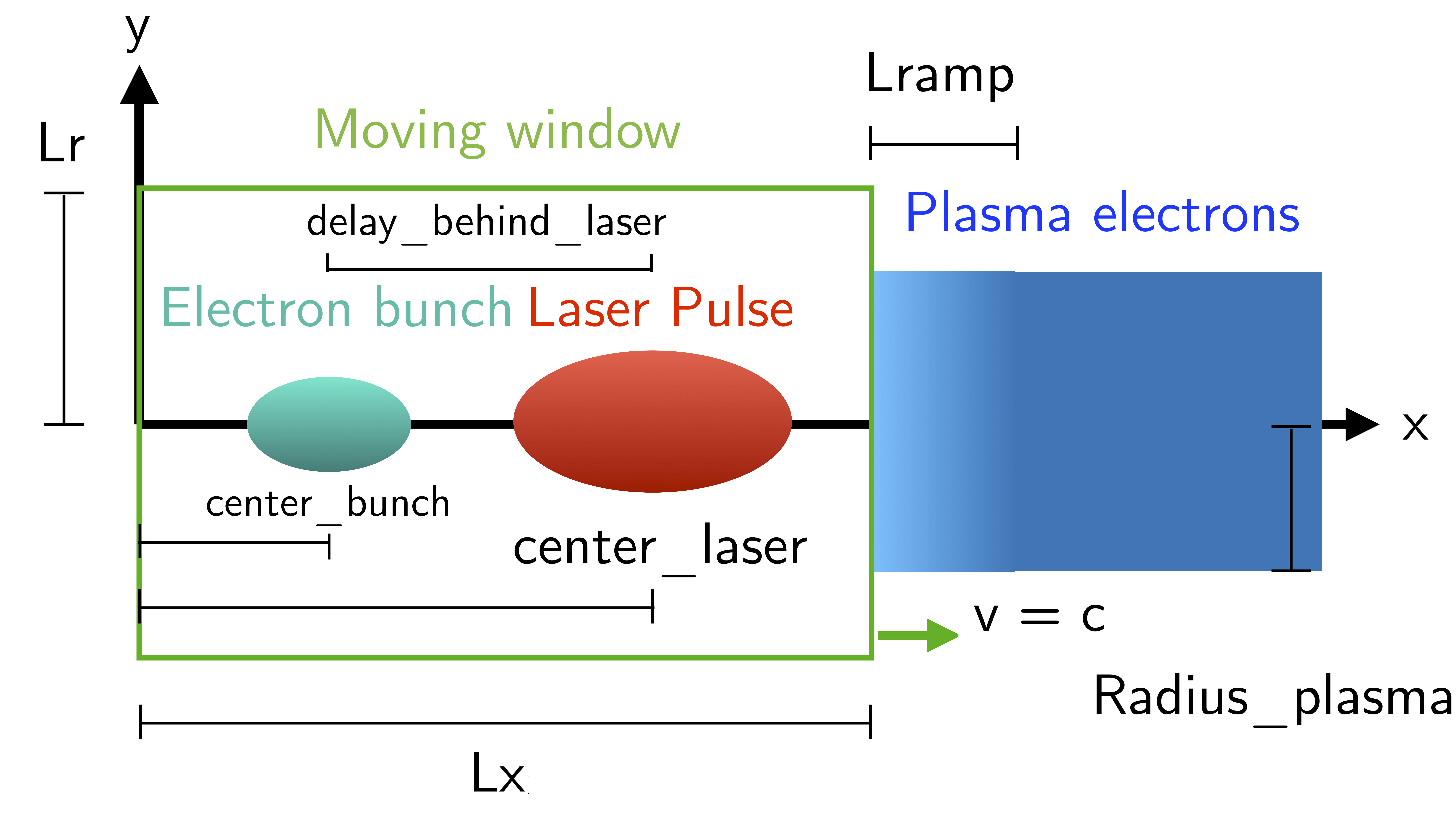
Fig. 6 Simulation Setup at the start of the simulation(s) in this Section (not to scale).
Exercise 12
Reading the InputNamelist.py, provide a description of the electron bunch at t = 0.
What is the total charge, the energy, the rms sizes along x, y, z, the rms energy spread, and the normalized emittance along the transverse planes?
How many macro-particles are modeling the electron bunch?
Where is the electron bunch placed in relation to the simulation window at the instant of time t = 0?
As the name suggests, this diagnostic block allows to track macro-particles
specified by their species name and some filter. Using a filter
(e.g., selecting only the particles with energy higher than 50 MeV) is
particularly useful when you have many particles in a Species,
like in the plasma of the namelist. In that case, not using a filter
would make this diagnostic computationally heavy and would store
the coordinates of too many particles. In the case of the bunch,
there is no need to specify a filter, since the number of macro-particles
is sufficiently small to be manageable. As you can see from the namelist,
in this diagnostic, we store the coordinates and momenta of the particles,
as well as their weight (from which their charge can be computed).
Exercise 13
Check that the simulation with the electron bunch has ended. This time the simulation will run a little longer.
Plot the 2D charge density (use Probe1) at timesteps=6000 and timesteps=10000
and play with the parameter vmax to be able to see the electron bunch
in the plasma wave.
Include these images in your answers.
Exercise 14 (advanced)
With the same simulation of Exercise 13, use the command
happi.multiPlot to plot in the same window
the longitudinal electric field Ex and the number density Rho/e
from Probe0 (1D diagnostic) at timesteps=6000 and timesteps=10000
(i.e. each window will contain the two quantities at a given timestep).
You may need to rescale the quantities (see Plot multiple lines in the same window in the Appendix).
Playing with multiplying factors in the plot you should be able
to clearly see where the electron bunch is placed in the plasma wave.
Include these images in your answers.
Exercise 15
With the same simulation of Exercise 13, run the script Compute_bunch_parameters.py in the simulation folder to read the electron bunch parameters.
For this purpose, from IPython you can use the command %run Compute_bunch_parameters.py timestep,
where timestep is the timestep you are interested in.
For example, the command %run Compute_bunch_parameters.py 10000 will return the electron bunch parameters the end of the simulation (i.e, at timestep = 10000).
What is the energy gain \(\Delta E\) you measure from the start (timestep = 0)
to the end of the simulation (timestep = 10000)?
What is the simulated propagation distance \(L\)?
From this information, estimate the average accelerating field \(E_{acc}\), including the derivation in your answer.
What is the absolute and relative rms energy spread at the beginning and at the end of the simulation?
Report all the electron bunch parameters at the start and at the end of the simulation.
Exercise 16 (advanced)
With the same simulation of Exercise 13, use the script Follow_electron_bunch_evolution.py to see how the bunch has evolved during
the simulation (%run Follow_electron_bunch_evolution.py
in IPython). The script reads the DiagTrackParticles output and
then computes some bunch quantities (rms size, emittance, energy)
at each available output iteration.
Include the resulting image in your answers.
From the evolution of the bunch energy, can you estimate the average accelerating field?
Compare this value to the one computed in Exercise 14.
Exercise 17 (advanced)
Create four new folders, sim1, sim2, sim3, sim4
where you will run four new simulation. In each simulation, the charge of the electron bunch will be changed to \(20, 40, 60, 80\) pC, respectively.
Warning: Do not forget the minus sign in the bunch charge, or the bunch will be made of positrons!
Adapt the commands you have used in Exercise 10 (happi.multiPlot commands) to plot the longitudinal electric
field Ex on axis (from Probe0) for the four cases. What do you observe? Include this plot in the answers.
Use the script
Compute_bunch_parameters.py
used for Exercise 14 to find the energy gain of the
electron bunch at timestep 10000 for each one of the four cases.
Can you explain how the deformation of the Ex waveform results in different final energies?
Hint: You can compare the Ex of the four simulations with multiPlot.
Include a plot of the energy gain of the bunch obtained for charges \(20, 40, 60, 80\) pC. You can use Python or any other language or program for this simple plot. For example, using Python:
import matplotlib.pyplot as plt
bunch=[20,40,60,80]
energy=[...,...,...,...] #replace by the energy values you obtained
fig = plt.figure()
plt.plot(bunch, energy, 'ro', markersize=10)
plt.xlabel(' Bunch charge [pC] ')
plt.ylabel(' ... ')
plt.show()
Exercise 18 (advanced)
Create other four folders, sim5, sim6, sim7, sim8,
where you will launch the simulation varying the bunch distance from the laser, changing the delay_behind_laser parameter (Set again the charge to \(60\) pC for all these simulations).
This parameter controls the distance between the electron bunch and the laser center, therefore its phase in the plasma wave behind the laser pulse.
For delay_behind_laser, try the values \(20, 22, 24, 26~ \mu m\).
What is the observed final energy for each of the four delay_behind_laser parameters?
Using happi.multiPlot (see Exercise 10), plot the longitudinal electric field Ex for the four simulations (show all curves in the same window and include the final image in your answers).
Again using happi.multiPlot, plot the electron number density Rho/e for the four simulations (show all curves in the same window and include the final image in your answers).
Include a plot with the delay_behind_laser on the horizontal axis and the energy gain on the vertical axis. You can use Python or any other language
for this simple plot (as you did for Exercise 16)
Exercise 19 (advanced)
For the same simulation of Exercise 13, using the TrackParticles diagnostic
and Probe diagnostic, write a script that takes as input variable an iteration number, i.e. timestep.
The script should plot in the same panel the longitudinal electric field Ex along the propagation axis x and a scatter plot of the electron bunch longitudinal phase space x and px
to show the particle longitudinal coordinate in the accelerating phase of Ex in that iteration.
The plot should report the correct units and labels in the axes.
In your answers, include the script and the output image using timesteps=6000 and timesteps=10000.
function using only dot markers.
Hint 1: To extract the propagation axis (in \(\mu m\)) and the Ex field (in GV/m) at the required timestep, you can use:
import happi
import numpy as np

S=happi.Open()

# in GV/m
Ex=np.asarray(S.Probe.Probe0("Ex",timesteps=timestep,units=["um","GV/m"]).getData())[0]

# in um
moving_x=np.linspace(0,S.namelist.Lx,num=S.namelist.nx)*S.namelist.c_over_omega0*1e6
x_window_shift = S.Probe.Probe0("Ex").getXmoved(timestep)*S.namelist.c_over_omega0*1e6

# in um
propagation_axis = moving_x + x_window_shift
Hint 2: To export the x (in \(\mu m\)) and px (in MeV/c) of the bunch macro-particles, you can use:
track_part = S.TrackParticles(species ="electronbunch",axes = ["x","px"],timesteps=timestep)

# x in um
x_bunch=track_part.getData()["x"]*S.namelist.c_over_omega0*1e6

# longitudinal momentum in MeV/c
import scipy.constants
electron_mass_MeV = scipy.constants.physical_constants["electron mass energy equivalent in MeV"][0]
px_bunch          = track_part.getData()["px"]*electron_mass_MeV
Hint 3: The Ex and px will have very different scales, so you will need
to use two y axes with different scales to see something meaningful.
With matplotlib you can do it through twinx.
Hint 4: Use a scatter plot for the x and px data of the bunch. For the propagation_axis and Ex plot, use a simple plot command.
Exercise 20 (advanced)
The accelerated electron bunch macro-particles do not have the same energies, so it is interesting to see the energy distribution or energy spectrum of the bunch particles before and after the acceleration.
Write a Python script to read the output of the DiagTrackParticles, and then use it to draw the energy spectrum (i.e. a histogram of the bunch macro-particle energies)
of the electron bunch (using MeV for the energies on the horizontal axis).
Provide the script and plot in the same window the energy spectrum at timesteps 0 and 10000 (the start and the end of the simulation).
The horizontal axis should be in MeV, while the vertical axis should be in pC/MeV.
Verify that the sum of the histogram bins multiplied by the energy bin width (i.e. the discrete version of the integral
in energy of the energy spectrum) is equal to the bunch charge and include also the
corrects units, labels and legend in the plot. Use an appropriate number of bins to see a meaningful image that shows the shape of the spectrum.
For reference, remember that the energy spectrum at the start of the simulation is a Gaussian, centered at the bunch initial energy.
Briefly comment on the differences in the energy spectrum at the start and at the end of the simulation.
Hint 1: You can extract the energy and charge of each macro-particle of the bunch at the desired timestep, using:
import happi
import numpy as np
import scipy.constants
import math
import matplotlib.pyplot as plt

S=happi.Open()

# Constants
c                       = scipy.constants.c         # lightspeed in vacuum,  m/s
epsilon0                = scipy.constants.epsilon_0 # vacuum permittivity, Farad/m
me                      = scipy.constants.m_e       # electron mass, kg
q                       = scipy.constants.e         # electron charge, C
electron_mass_MeV       = scipy.constants.physical_constants["electron mass energy equivalent in MeV"][0]

lambda0                 = S.namelist.lambda0        # laser central wavelength, m
conversion_factor_length= lambda0/2./math.pi*1.e6   # from c/omega0 to um, corresponds to laser wavelength 0.8 um
nc                      = epsilon0*me/q/q*(2.*math.pi/lambda0*c)**2 # critical density in m^(-3)

# extract data from TrackParticles
track_part = S.TrackParticles(species ="electronbunch",axes = ["w","px","py","pz"],timesteps=timestep)

# extract charge in pC
conversion_factor_charge= q * nc * (conversion_factor_length*1e-6)**3 * 10**(12)
charge_bunch_pC=track_part.getData()["w"]*conversion_factor_charge

# extract momenta in MeV/c
px_bunch=track_part.getData()["px"]
py_bunch=track_part.getData()["py"]
pz_bunch=track_part.getData()["pz"]

p_bunch = np.sqrt((px_bunch**2+py_bunch**2+pz_bunch**2))

# electron energy in MeV
E_bunch = np.sqrt((1.+p_bunch**2))*electron_mass_MeV
Hint 2: you can use the matplotlib function numpy.histogram to compute a
histogram of the macro-particles energies and the bins/edges of the horizontal axis.
The energy spectrum is a histogram of the macro-particle energies using their charge as statistical weight.